XYZFlow: When More Context Beats Fewer Steps

Paper: 2608.12276 Authors: Jinxiu Liu, Xuanming Liu, Kangfu Mei, Yandong Wen, Weiyang Liu Categories: cs.CV

The Gap

The fast-sampling literature has mostly converged on one recipe: train a good slow model, then compress it. Progressive distillation, consistency models and LCM, DMD, rectified-flow reflow — all of them need a teacher, and all of them inherit the teacher’s failure modes plus a distillation gap on top. Shortcut models broke that dependency by training a single network conditioned on both time t and step size d, with a self-consistency constraint that one jump of size 2d should equal two jumps of size d. No teacher, few steps, one training run.

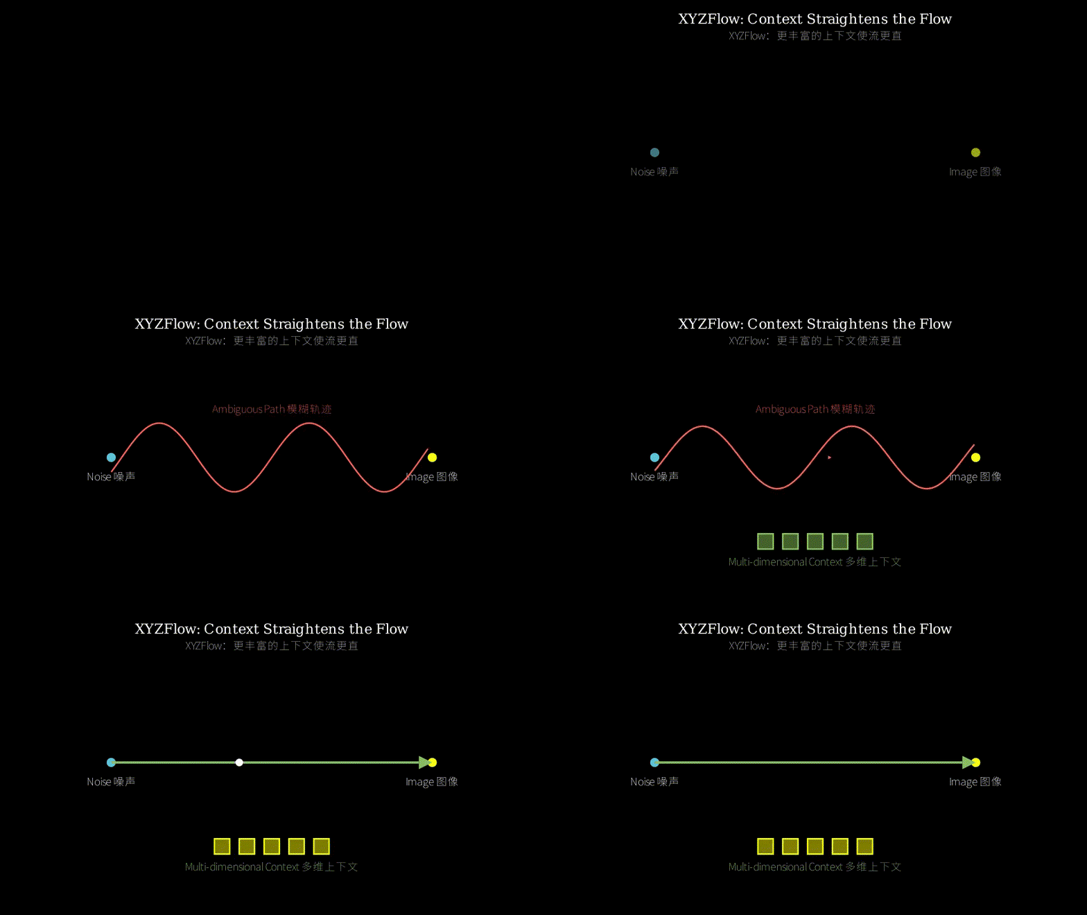
But shortcut models hit a wall that is easy to state and hard to fix. When you ask a network to jump a long distance along a probability path, the state you are jumping from is compatible with many different endpoints. The regression target is therefore an average over plausible endpoints, and averaging images gives you exactly what everyone observes: soft edges, washed texture, mode collapse toward the mean. The usual response is to make the model bigger or take a couple more steps.

XYZFlow’s bet is that this is a conditioning problem, not a capacity problem. The path is ambiguous because the model is told too little about it: it sees only the current noisy state, Markov-style, and nothing about where it came from or what its neighbors decided. Add the right conditioning and the path becomes identifiable — which the paper frames as *autoregressive modeling being implicit flow straightening.

[PROBLEM] high fidelity needs 50+ steps; few-step methods
          distill a teacher and inherit its ceiling
     |
     v
[WHY IT BREAKS] one big jump from (x_t, t, d) is compatible
                with many endpoints  ==>  target is an
                average  ==>  blur / lost detail
     |
     v
[ASSUMPTION] ambiguity comes from missing context, not from
             missing parameters.  richer conditioning
             == more identifiable path == straighter flow
     |
     +-------------------+--------------------+
     v                   v                    v
[base axis: d]     [Y: temporal]         [X: spatial]
 shortcut self-     non-Markovian         Next Shortcut
 consistency        conditioning on       Prediction: patch
 (d + d == 2d)      the whole denoise     n conditioned on
                    history               traces of patch <n
     |                   |                    |
     +-------------------+--------------------+
                         v
[EVIDENCE] 7.2x - 8.5x speedup over the teacher with
           competitive FID; NSP dominates both
           param-scaling and step-scaling on the
           quality-vs-latency curve
                         |
                         v
[CONCLUSION] scale the conditioning axes, not the step count
             or the parameter count

The Increment

One sentence: Before, making generation fast meant squeezing a teacher into fewer steps and eating the quality loss; after, it means keeping few steps but feeding the sampler far more context — its own denoising history and its neighbors’ trajectories — so that each big jump is well-determined in the first place.

Core Mechanism

Start from the shortcut-model backbone: a velocity network v_theta takes (x_t, t, d) and predicts a jump, trained with a flow-matching loss plus the self-consistency loss that ties one 2d step to two d steps. XYZFlow keeps that skeleton and widens the conditioning bundle along two orthogonal axes.

Temporal scaling (Y) makes sampling non-Markovian. In a standard sampler each step throws away everything except the current latent. Here the previously visited states are cached and fed back in as additional conditioning, so at step t the network sees x_t and the trail x_1, x_{1-d}, ..., x_{t+d}. That trail encodes the heading and curvature of the trajectory so far, which is precisely the information that disambiguates where the path is going. Note the cost profile: this is nearly free at inference because those states already exist — you are reusing computation you had thrown away.

Spatial scaling (X) is the more aggressive move, called Next Shortcut Prediction. Instead of denoising the whole image jointly, patches are generated in sequence, and each new patch is conditioned on the denoising trajectories of the patches that came before it — not merely their finished pixels. That distinction is the whole point. Handing over the final clean patch is ordinary patch-wise autoregression; handing over the entire shortcut trace tells the new patch how its neighbor got there, at every noise level, which lets it align its own path from the very first jump rather than only agreeing at the end. Together with the step-size axis inherited from shortcut models, that gives the three conditioning dimensions the name gestures at (the paper’s abstract only names two, so read the third as the shortcut d axis).

  conditioning bundle fed to v_theta at each jump:
  +-------------------------------------------------------+
  |  x_t     current noisy latent            (base)       |
  |  t       time                            (base)       |
  |  d       shortcut step size              (Z axis)     |
  |  H       own visited states x_1 ... x_(t+d)   (Y axis)|
  |  S       full denoise traces of earlier patches (X)   |
  +-------------------------------------------------------+
                      |
                      v
                [ transformer ]
                      |
                      v
        v_theta  ==>  x_(t-d) = x_t - d * v_theta
                      |
        losses: flow matching  +  self-consistency
                (one 2d jump == two chained d jumps)

  Next Shortcut Prediction, patch order p1 -> p4:

    p1 : [t, d, x_t, H1              ]  ==> trace T1
    p2 : [t, d, x_t, H2, T1          ]  ==> trace T2
    p3 : [t, d, x_t, H3, T1, T2      ]  ==> trace T3
    p4 : [t, d, x_t, H4, T1, T2, T3  ]  ==> trace T4

    what crosses the arrow is the *trace*, not the pixels

The metaphor: a convoy driving with dead reckoning. Each patch is a car; the clean image is the destination; the velocity network is the driver’s judgment; the step size d is how far you dare drive between glances at the map.

A vanilla few-step sampler is an amnesiac driver: at each glance they know only their current GPS coordinate, nothing about the road they just came down. From a single point, a hundred destinations are plausible, so if you ask them to drive a long stretch blind they aim at the average of all of them and end up in a field. Temporal scaling hands that driver a breadcrumb trail of every point they have passed. Now they can read off their heading and how the road is curving, and a long blind stretch becomes a safe extrapolation instead of a guess — which is why bigger steps stop hurting.

Spatial scaling turns one car into a convoy on radio. The lead car drives first, and rather than just parking and texting back its final address, it broadcasts its whole route: every turn, at every stage. The second car starts driving already knowing the shape of the road ahead, so it doesn’t have to rediscover it and doesn’t drift out of formation. That is Next Shortcut Prediction, and it explains both the win and the cost: formation is tight (coherent, detailed images) but the cars leave one after another, so the convoy is inherently serial.

Key Concepts

• Trajectory ambiguity (and why averaging blurs): Imagine a very noisy patch of gray fuzz. Consistent with it are a cat’s ear, a leaf, a shirt collar. A network trained by least squares to name the clean answer in one shot cannot pick; the loss is minimized by outputting the pixel-wise mean of all three, which looks like nothing in particular — soft, smudgy, mid-gray. Many small steps avoid this because each step only has to resolve a sliver of ambiguity, letting the choice be made gradually. XYZFlow’s move is to kill the ambiguity with side information instead of with extra steps: if you also know the trail that led here and what the neighboring region turned out to be, “cat’s ear” becomes the only sensible continuation, and one big step is safe.

• Shortcut model / self-consistency: A normal flow model learns the instantaneous direction at each point, valid only for infinitesimal steps. A shortcut model takes step size as an *input, so one network represents a family of samplers from 128 steps down to 1. The trick that makes it trainable without a teacher: for any state, taking two steps of size d and one step of size 2d must land in the same place. That constraint propagates knowledge from cheap-and-accurate small steps up to expensive-and-crude big steps inside a single training run — a bootstrap, not a distillation.

• Autoregression as implicit flow straightening: “Straightening” a flow means making noise-to-data paths closer to straight lines, since straight lines can be traversed in one step exactly. Reflow does this by retraining on the model’s own noise-data pairs. The paper’s reframing: conditioning on more context does the same thing for free, because a path only looks curved and wiggly when you are uncertain which path you are on. Pin down the context and the *effective path — the conditional expectation the network has to regress — becomes much straighter. Autoregression is thus a straightening device that happens to be spelled as a factorization.

Framework Shift

Before (mainstream approach):          After (this paper):

 [ teacher, 50 steps ]                 [ one model, no teacher ]
          |                                      |
      distill / reflow                cond = (x_t, t, d, H, S)
          |                                      |
          v                                      v
 [ student: x_t --> x_0 ]              x_t -o--o--o-> x_0
   memoryless single map                    ^  ^  ^
   whole image at once                      |  |  |   (Y)
                                       own history fed back
   many endpoints fit                       + (X) sideways:
   -> averaged target                  p1 trace -> p2 -> p3
   -> soft, low detail
                                       path is identifiable,
   quality ceiling <= teacher          so big jumps are exact
   axis of improvement:                axis of improvement:
     fewer steps, more params            more conditioning dims

From step-compression to context-expansion, the core shift is treating few-step generation as an identifiability problem solved by conditioning, rather than a compression problem solved by distillation.

Expert Assessment

Caveat up front: I am reading from the abstract, so my read on the numbers is provisional — the specific FID values, datasets, and latency methodology are where this paper will live or die, and they are not in front of me.

Problem choice: Genuine, and well-diagnosed. Teacher dependence is the real structural weakness of the distillation family, and the averaging pathology of large-jump regression is the correct explanation for why teacher-free few-step models look soft. It is also a crowded neighborhood: MAR/Fluid-style continuous autoregression, “next-X prediction” variants, rolling diffusion, and AR-diffusion hybrids have all been circling the “autoregression complements diffusion” idea. The framing of autoregression as implicit straightening is the freshest thing here, and it is a framing rather than a theorem.

Method maturity: Mostly clever, partly brute force. Temporal scaling is elegant and nearly free — it generalizes self-conditioning from one previous prediction to the full history, and the cached states are already sitting in memory. Spatial scaling is where I get uneasy, because sequential patch decoding reintroduces exactly the serial latency that few-step sampling exists to remove. The paper’s own claim that NSP beats step-reduction on the quality-latency curve is a bet that KV-cached patch passes are cheaper than extra full-image passes; plausible at low patch counts, fragile as resolution grows. Two simpler things deserve explicit comparison: MeanFlow, which attacks the same ambiguity by parameterizing average velocity within one network and no history at all, and plain self-conditioning, a one-line trick that captures a chunk of the temporal axis. Also unaddressed in the abstract: non-Markovian conditioning at inference means the model consumes its own past states, so exposure bias and error compounding are live risks that need a teacher-forcing or noise-augmentation story.

Experimental integrity: The headline “7.2-8.5x teacher speedup” is a soft metric — it is measured against the authors’ own teacher, so it moves with how slow that teacher was configured to be, and “competitive FID” is doing real work in that sentence. What I would want: absolute wall-clock at matched FID against LCM/DMD/shortcut/MeanFlow, iso-FLOPs and iso-parameter comparisons for the NSP-vs-model-scaling claim, and the same claim at 512px, where sequential patch decode should degrade. Scaling comparisons are notoriously sensitive to how much tuning each arm received, so that headline claim is the one I would probe hardest.

Writing quality: “Identifiable” and “expressivity” are doing heavy lifting with no formal backing visible; even a toy two-mode example with a closed-form conditional expectation would convert the central intuition from rhetoric into an argument. The branding is also a tell — a name promising three dimensions while the abstract names two suggests the third axis is thin. The section I would rewrite is the latency accounting: make the serial cost of NSP explicit and quantified, because a skeptical reader’s first instinct is that patch-wise autoregression is trading the win right back.

Verdict: weak accept — the reframing is genuinely useful and the temporal axis is a cheap, transferable win, but the central quality-latency claim rests on comparisons that are easy to tilt and that I cannot check from the abstract.

Takeaways

• Stop throwing away your denoising history. If you already run a multi-step DiT sampler, the previous latents are free context. Feeding them back as extra tokens is a small architectural change with a plausible quality-per-step payoff, and it subsumes self-conditioning as a special case.
• Pass trajectories between autoregressive units, not outputs. This is the transferable idea. In video, hand the next frame the previous frames’ per-noise-level traces instead of just the finished frames; likewise for 3D tiles, long audio, or tiled super-resolution. Sharing *how a neighbor was produced aligns paths from the first step rather than patching up disagreement at the end.
• A new diagnostic reflex: when a few-step student comes out blurry, ask whether the target is ambiguous before assuming the model is too small. Averaged-target blur and under-capacity blur look similar and have completely different fixes; conditioning is usually the cheaper one to try.
• Bootstrap instead of distill. The self-consistency trick (one 2d step equals two d steps) is a general pattern for transferring competence from a cheap accurate regime to an expensive crude one inside a single model — applicable well beyond image flows.
• Report the curve, not the point. Comparing quality-vs-latency curves rather than FID at a fixed step count is the right evaluation posture, and it is what makes the paper’s most interesting claim legible in the first place. Just hold others to the same standard you hold yourself.