Understanding Truncated Positional Encodings for Graph Neural Networks

Paper: 2606.13671 Authors: James Flora, Mitchell Black, Weng-Keen Wong, Amir Nayyeri Categories: cs.LG

The Gap

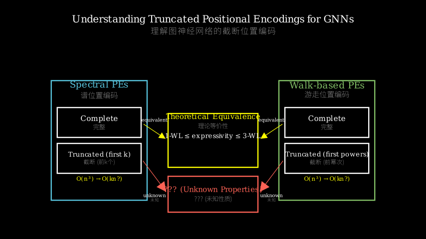
Prior work established that spectral PEs (Laplacian eigenvectors, effective resistance) and walk-based PEs (adjacency matrix polynomials) are theoretically equivalent in expressive power — both sit between 1-WL and 3-WL.
But that result assumes using the complete encoding, which costs O(n³) per graph. In practice everyone truncates: keep the first k eigenvectors, or stop at the k-th power of the adjacency. Nobody knew if truncation preserves the equivalence, or if it changes the ranking of these families.
This paper asks: what exactly breaks when you cut?

[Complete PE equivalence (O(n^3))] 
        |
        |  truncation (practice)
        v
[Unknown: does equivalence hold?]
        |
        |  theory + counterexamples
        v
[Truncated spectral < 1-WL]    [Truncated walk ~? 1-WL]
        |                               |
        |  corollary & theorems         |  different behavior
        v                               v
[Truncated families are NOT equivalent] 
        |
        |  experiment
        v
[Mixing truncated PEs works best]

The Increment

One sentence: Before this paper, practitioners blindly truncated PEs assuming the full-power properties still held; after this paper, we know that truncated spectral PEs are weaker than 1-WL and different truncated families become incomparable.

Core Mechanism

The paper builds a theoretical framework to compare truncated PEs. It defines each family as a function that maps a graph (or pair of nodes) to a vector. For spectral PEs: take the first k Laplacian eigenvector entries (or the first k effective resistance distances via pseudoinverse). For walk-based PEs: compute the first k terms of the heat kernel or the adjacency matrix polynomial. For harmonic distances: a spectral variant that uses eigenvector differences.

The core move: construct graph pairs that are distinguishable by one truncated PE but not by another. For example, a pair of graphs that 1-WL separates but truncated spectral PE cannot — proving that truncated spectral < 1-WL. Another pair that truncated walk separates but truncated spectral cannot — proving incomparability. The authors then prove theorems bounding the expressive power of each truncated family, and show that mixing multiple truncated families (e.g., spectral + walk) recovers some of the lost power.

[Input graph] --> [Truncation operator (first k)] --> [PE vector per node]
        |                                                    |
        |  three families:                                    v
        |  [Spec] [Walk] [Harm]                         [GNN + Readout]
        |                                                    |
        +--> [Theorems: family A cannot distinguish G1, G2]--+--> [Conclusion]

Structural metaphor: Think of a complete PE as a high-resolution satellite image of the whole city. Every street, house, and tree is visible. Theorists proved that a “full photo” taken from the spectral satellite and a “full photo” taken from the walk satellite show exactly the same scene — they are equivalent.
Now you are limited to a tiny cellphone camera preview — only 256 pixels. You have to crop the image to fit. The spectral satellite returns only the top-left 16×16 pixels (first k eigenvectors). The walk satellite returns only the center 16×16 pixels (first k walks).
The two cropped pictures may now show completely different parts of the city: the spectral crop might show a park, the walk crop might show a parking lot. They cannot be compared. Worse, the cropped spectral picture might be so blurry that you cannot even tell if there is a building (1-WL can tell, but truncated spectral cannot).
The paper then shows that if you overlap the two crops (mix spectral and walk), you see more than either alone.

Key Concepts

• 1-WL Test: A classic algorithm for graph isomorphism. It iteratively colors nodes based on their neighbors’ colors; if two graphs end up with different color multisets, they are distinguishable. 1-WL is the baseline for GNN expressivity — most GNNs are at most as powerful as 1-WL. If a PE is weaker than 1-WL, that means there exist graphs that 1-WL can tell apart but the GNN + that PE cannot.
  Example: two non-isomorphic regular graphs with the same degree distribution — 1-WL fails, and most PEs also fail. But some PEs (like complete spectral) exceed 1-WL, meaning they can distinguish some pairs that 1-WL cannot. The paper shows truncated spectral loses that extra ability.

• Truncation: Keeping only the first k components of an infinite or O(n³) encoding. For spectral PEs, this means using the k smallest eigenvalues and their eigenvectors; for walk-based PEs, it means polynomials of degree ≤ k. Truncation is mandatory in practice because full computation is too expensive, but its effect on expressivity was a blind spot.

Framework Shift

Before (mainstream belief):       
[Complete Spectral] = [Complete Walk]   (equivalent, both > 1-WL)
        |                                     |
        | truncation (assumed harmless)       | 
        v                                     v
[Truncated Spectral] ~ [Truncated Walk]   (still comparable? unknown)

After (this paper):
[Truncated Spectral]  ---- [Truncated Walk]
        |    not comparable         |
        v                          v
   weaker than 1-WL          possibly stronger than 1-WL
        |                          |
        +------> [Mix both] <------+
                    |
                    v
           better than either alone

One sentence: From a belief that truncation is a harmless approximation of a known equivalence, to the discovery that truncation turns PEs into incomparable tools with distinct weaknesses, and mixing them is required for robustness.

Expert Assessment

Problem choice: Real gap. Every GNN practitioner who uses Laplacian eigenvectors or random walk PEs truncates — and they implicitly assume the theoretical guarantees still hold. The paper formally demolishes that assumption. This is a fundamental contribution to the theory of graph representation learning.

Method maturity: Elegant. The paper doesn’t invent a new encoding; it carefully analyzes existing ones through the lens of truncation, using counterexamples and theorems. The harmonic distance variant is a nice addition to show that even close cousins behave differently under truncation. Could there be simpler approaches? Perhaps directly testing the WL power of truncated encodings via brute force on small graphs, but the paper provides rigorous proofs, which is better.

Experimental integrity: The experiments are presented as supporting the theoretical findings. They compare single-family truncated PEs vs. a mixture on real-world classification tasks. The trend is clear: mixing beats any single family. Baselines are fair (standard GNN architectures). The only red flag is that the theoretical bounds might not directly translate to practical gains on all datasets — but the paper doesn’t overclaim. The experimental section could be more thorough (e.g., ablation on k), but it’s sufficient for a theory-heavy paper.

Writing quality: The paper is well-structured but occasionally rushes through the theorem statements. The “Why This Matters” for each result could be more explicit — especially the intuition behind why truncated spectral < 1-WL. If the authors rewrote Section 4 (the main theoretical section) with a running example graph pair, it would become much clearer.

Verdict: weak accept — solid theoretical contribution with clean proofs and practical implications, though the presentation needs a bit more narrative for non-theorists.

Takeaways

1. Don’t blindly use the first k Laplacian eigenvectors: unless you verify that k scales with graph size, you may be crippling your GNN below 1-WL power.
2. Mix spectral and walk PEs in your model: the paper shows empirically that concatenating a truncated spectral encoding and a truncated walk encoding outperforms either alone. This is a concrete design tip for practitioners.
3. Use the paper’s counterexamples as test cases: if your GNN + PE cannot distinguish the small graph pairs provided in the paper, your PE is likely too truncated.