Paper: 2605.20179 Authors: Zhiben Chen, Youpeng Zhao, Yang Sui, Jun Wang, Yuzhang Shang Categories: cs.CL
The Gap
Diffusion LLMs (dLLMs) with mixture-of-experts (MoE) architectures promise better parallelism than autoregressive models, but deploying them on resource-constrained devices hits a wall. Existing solutions borrowed from AR models fail here: naive expert offloading (moving unused experts to CPU) causes massive I/O overhead because experts get swapped constantly, while keeping all experts on GPU exhausts memory. The core problem is that AR methods treat each token independently, but dLLMs generate entire blocks through iterative diffusion steps—a fundamentally different temporal structure that existing systems ignore.
Problem: MoE dLLMs too large for single GPU
    |
    v
Observation: Diffusion steps within a block reuse similar experts
    |
    v
Assumption: Expert activation patterns are temporally stable
    |
    v
Method: Refresh experts at intervals, not every step
    |
    v
Evidence: 1.4-1.5x speedup with zero accuracy loss
    |
    v
Conclusion: Temporal stability enables I/O-efficient offloading
The Increment
One sentence: Before TIDE, MoE dLLM inference either thrashed I/O by swapping experts constantly or ran out of GPU memory; after TIDE, we exploit diffusion’s temporal stability to refresh experts only when needed, achieving lossless speedup.
Core Mechanism
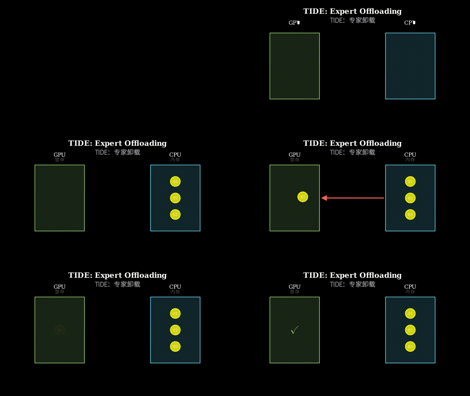
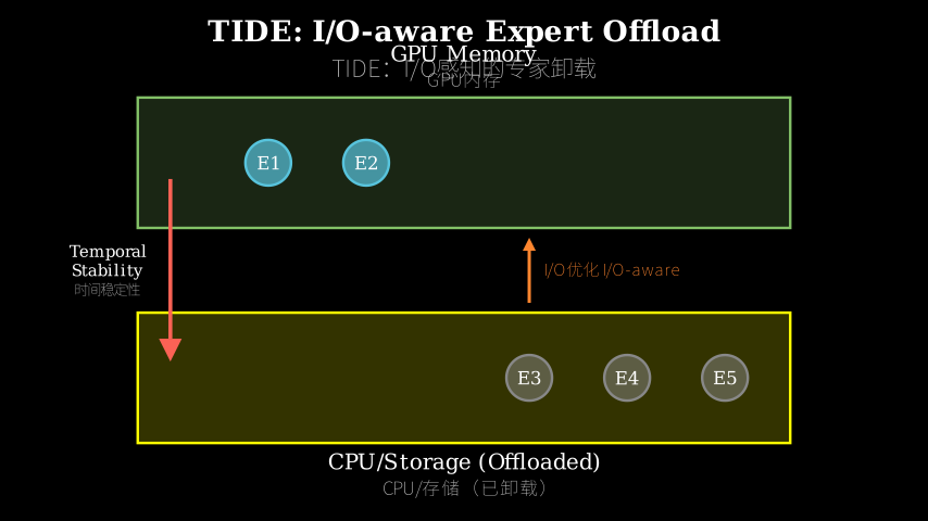
TIDE operates on a simple insight: during the diffusion process that generates a single block, the same experts tend to be activated repeatedly across consecutive steps. Instead of loading experts from CPU for every diffusion step (expensive I/O), TIDE keeps a working set of experts on GPU and refreshes them only at calculated intervals.
The system has three components: (1) an expert activation tracker that monitors which experts are used during diffusion, (2) an interval calculator that solves an optimization problem to determine when to refresh the expert set, balancing I/O cost against the risk of missing an expert, and (3) a prefetching scheduler that loads the next interval’s experts while the current interval is still computing. The optimization formulation minimizes total latency by trading off PCIe transfer time against CPU fallback computation time.
Data flows like this: at the start of each interval, TIDE loads a predicted set of experts onto GPU. During the interval’s diffusion steps, if an expert is needed but not present, the system falls back to CPU computation for that expert (slow but correct). At interval boundaries, TIDE analyzes recent activation patterns, solves the optimization to pick the next interval length and expert set, then prefetches those experts while the current interval finishes.
Structural metaphor: Think of TIDE as a library reading room with limited desk space. You’re working through a multi-chapter book (the diffusion process), and each chapter references certain reference books (experts). Instead of running to the stacks (CPU) every time you need a citation (expert call), you predict which references you’ll need for the next few pages (interval) and keep them on your desk (GPU). Occasionally you guess wrong and have to make a quick trip to the stacks (CPU fallback), but most of the time you work uninterrupted. Every few pages, you pause, look at which references you actually used, and swap out your desk books for the next predicted set. The optimization problem is: how many pages should you read before swapping? Too short and you waste time swapping; too long and you make too many trips to the stacks.
Key Concepts
-
Temporal stability in diffusion: In autoregressive generation, each token is independent—predicting token 50 doesn’t tell you much about token 51’s expert needs. But diffusion LLMs generate a block by iteratively refining it over multiple steps, like an artist sketching then adding detail. Early steps might activate “structure” experts, middle steps activate “refinement” experts, and late steps activate “polishing” experts. Within a short window (say, 5 consecutive diffusion steps), the same experts fire repeatedly because the model is working on the same semantic content. This isn’t a guarantee—it’s a statistical tendency that TIDE exploits. The paper measures this by tracking expert activation overlap across consecutive steps and finds high correlation.
-
Interval-based refresh: Instead of deciding “load expert X or not” at every step, TIDE decides “for the next N steps, keep experts {A, B, C} on GPU.” N is the interval length. At the end of N steps, TIDE re-evaluates: which experts were actually used? Which will likely be needed next? Then it swaps the GPU expert set. The interval length is not fixed—it’s computed per-interval by solving an optimization that considers: (1) how much I/O time a swap costs, (2) how much CPU fallback time we’ll incur if we guess wrong, (3) how stable recent expert patterns have been. Short intervals mean frequent swaps (high I/O cost). Long intervals mean more CPU fallbacks (high compute cost). The optimization finds the sweet spot.
-
I/O-aware scheduling: The optimization problem TIDE solves is: minimize
total_time = (num_intervals × swap_time) + (num_fallbacks × fallback_time). Swap time is the PCIe transfer cost to move experts between CPU and GPU. Fallback time is the cost of running an expert on CPU when it’s not on GPU. The decision variables are: (1) interval length, (2) which experts to keep on GPU. TIDE formulates this as a mathematical program and solves it using historical activation data from previous intervals. The “I/O-aware” part means the solution explicitly accounts for hardware characteristics—PCIe bandwidth, CPU vs GPU compute speed—rather than using a heuristic.
Framework Shift
Before (AR-based offloading):        After (TIDE):

Step 1: [GPU: E1,E2] -> need E3      Interval 1 (steps 1-5):
        swap E1 out, E3 in            [GPU: E1,E2,E3]
        |                             step 1: use E1,E2
        v                             step 2: use E2,E3
Step 2: [GPU: E2,E3] -> need E1      step 3: use E1,E3
        swap E3 out, E1 in            step 4: use E2,E3
        |                             step 5: use E1,E2
        v                                 |
Step 3: [GPU: E1,E2] -> need E3           v
        swap E1 out, E3 in            Refresh: analyze, optimize
        ...                               |
                                          v
(thrashing: constant swaps)           Interval 2 (steps 6-9):
                                      [GPU: E2,E3,E4]
                                      ...

                                      (batched swaps: amortized cost)
One sentence: From per-step reactive swapping to interval-based predictive batching, the core shift is exploiting temporal locality to amortize I/O overhead.
Expert Assessment
Problem choice: Real gap. MoE dLLMs are emerging as a serious alternative to AR models, and deployment on consumer hardware is a genuine bottleneck. The observation that diffusion’s iterative structure creates temporal stability is non-obvious and well-motivated. This sits at the intersection of two trends: scaling via MoE and exploring non-AR architectures.
Method maturity: The core idea—exploit temporal stability—is elegant. The interval optimization is solid engineering but not groundbreaking theory. One concern: the method assumes activation patterns are stable enough to predict, but the paper doesn’t deeply explore failure modes. What happens in highly diverse generation tasks where expert usage is chaotic? The fallback to CPU is a safety net, but if fallback rate is high, the speedup evaporates. The paper shows good results on two models, but generalization to other dLLM architectures is unclear.
Experimental integrity: Baselines are fair—comparing against naive offloading and a recent AR-based method (PowerInfer). The 1.4-1.5× speedup is respectable but not dramatic. Critically, the paper claims “lossless” optimization, meaning zero accuracy degradation, which is verified. However, the experiments are limited to two model sizes (mini and flash) on specific hardware (single GPU-CPU setup). Scaling behavior with larger models or multi-GPU setups is unexplored. The ablation studies are thorough, showing the impact of interval length and expert set size.
Writing quality: The paper is well-structured but dense. The optimization formulation in Section 3.2 is heavy on notation without enough intuition-building first. A reader unfamiliar with scheduling problems will struggle. The related work section is comprehensive but could be tighter. The biggest missed opportunity: no discussion of when TIDE fails. Every method has a regime where it breaks down—acknowledging this would strengthen credibility.
Verdict: weak accept — Solid engineering contribution with clear practical value, but limited theoretical depth and narrow experimental scope. The temporal stability insight is valuable, but the paper doesn’t push hard enough on understanding its boundaries.
Takeaways
Transferable idea: The interval-based refresh strategy generalizes beyond dLLMs. Any system with temporal locality in resource access (caching, prefetching, memory management) can benefit from formulating the refresh schedule as an optimization problem that balances swap cost against miss cost. The key is: don’t react to every access—batch decisions and amortize overhead.
Concrete technique: The mathematical programming formulation for interval length is reusable. If you’re building a system that swaps resources between fast and slow storage, steal this: model total cost as (swap_frequency × swap_cost) + (miss_rate × miss_cost), then solve for the interval that minimizes it. The paper’s formulation accounts for hardware characteristics (PCIe bandwidth, compute speed), which is often overlooked in heuristic-based systems.
Framing shift: The “lossless optimization” framing is powerful for deployment-focused work. By guaranteeing zero accuracy loss, TIDE sidesteps the usual training-inference tradeoff and positions itself as a drop-in replacement. If you’re working on inference optimization, consider whether your method can be lossless—it’s a strong selling point for practitioners who can’t afford accuracy degradation.
论文: 2605.20179 作者: Zhiben Chen, Youpeng Zhao, Yang Sui, Jun Wang, Yuzhang Shang 分类: cs.CL
缺口
带有混合专家(MoE)架构的扩散 LLM(dLLM)承诺比自回归模型有更好的并行性,但在资源受限设备上部署时遇到瓶颈。
从自回归模型借来的现有方案在这里失效:朴素的专家卸载(将未使用的专家移到 CPU)会导致巨大的 I/O 开销,因为专家被频繁交换;而将所有专家保留在 GPU 上又会耗尽内存。
核心问题在于,自回归方法独立处理每个 token,但 dLLM 通过迭代扩散步骤生成整个块——这是一种根本不同的时序结构,现有系统忽略了这一点。
问题:MoE dLLM 对单 GPU 来说太大
    |
    v
观察:块内的扩散步骤重用相似的专家
    |
    v
假设:专家激活模式具有时序稳定性
    |
    v
方法:按间隔刷新专家,而非每步都刷新
    |
    v
证据:1.4-1.5 倍加速,零精度损失
    |
    v
结论:时序稳定性使 I/O 高效卸载成为可能
增量
一句话:TIDE 之前,MoE dLLM 推理要么因频繁交换专家而 I/O 抖动,要么耗尽 GPU 内存;TIDE 之后,我们利用扩散的时序稳定性,仅在需要时刷新专家,实现无损加速。
核心机制
TIDE 基于一个简单的洞察:在生成单个块的扩散过程中,相同的专家往往在连续步骤中被重复激活。
TIDE 不是在每个扩散步骤都从 CPU 加载专家(昂贵的 I/O),而是在 GPU 上保留一组工作专家,仅在计算出的间隔处刷新它们。
系统有三个组件:(1)专家激活跟踪器,监控扩散期间使用了哪些专家;(2)间隔计算器,求解优化问题以确定何时刷新专家集,在 I/O 成本和错过专家的风险之间取得平衡;(3)预取调度器,在当前间隔仍在计算时加载下一个间隔的专家。
优化公式通过权衡 PCIe 传输时间和 CPU 回退计算时间来最小化总延迟。
数据流动如下:在每个间隔开始时,TIDE 将预测的专家集加载到 GPU。
在间隔的扩散步骤期间,如果需要某个专家但它不在 GPU 上,系统会回退到 CPU 计算该专家(慢但正确)。
在间隔边界,TIDE 分析最近的激活模式,求解优化以选择下一个间隔长度和专家集,然后在当前间隔结束时预取这些专家。
核喻:把 TIDE 想象成一个桌面空间有限的图书馆阅览室。
你正在读一本多章节的书(扩散过程),每章引用某些参考书(专家)。
你不是每次需要引用(专家调用)时都跑到书库(CPU),而是预测接下来几页(间隔)需要哪些参考书,并把它们放在桌上(GPU)。
偶尔你猜错了,不得不快速跑一趟书库(CPU 回退),但大多数时候你不受干扰地工作。
每隔几页,你暂停,看看实际使用了哪些参考书,然后为下一个预测集交换桌上的书。
优化问题是:交换前应该读多少页?太短会浪费时间交换;太长会跑太多次书库。
关键概念
- 扩散中的时序稳定性:在自回归生成中,每个 token 是独立的——预测第 50 个 token 不会告诉你太多关于第 51 个 token 的专家需求。
但扩散 LLM 通过多个步骤迭代细化来生成一个块,就像艺术家先画草图再添加细节。
早期步骤可能激活”结构”专家,中期步骤激活”细化”专家,后期步骤激活”润色”专家。
在一个短窗口内(比如 5 个连续扩散步骤),相同的专家会重复触发,因为模型在处理相同的语义内容。
这不是保证——而是 TIDE 利用的统计趋势。
论文通过跟踪连续步骤间的专家激活重叠来测量这一点,发现高度相关性。
- 基于间隔的刷新:TIDE 不是在每步决定”加载专家 X 还是不加载”,而是决定”在接下来的 N 步中,在 GPU 上保留专家 {A, B, C}”。
N 是间隔长度。
在 N 步结束时,TIDE 重新评估:实际使用了哪些专家?接下来可能需要哪些?然后交换 GPU 专家集。
间隔长度不是固定的——它是通过求解优化来按间隔计算的,该优化考虑:(1)交换的 I/O 时间成本,(2)如果猜错会产生多少 CPU 回退时间,(3)最近的专家模式有多稳定。
短间隔意味着频繁交换(高 I/O 成本)。
长间隔意味着更多 CPU 回退(高计算成本)。
优化找到最佳点。
- I/O 感知调度:TIDE 求解的优化问题是:最小化
总时间 = (间隔数 × 交换时间) + (回退数 × 回退时间)。
交换时间是在 CPU 和 GPU 之间移动专家的 PCIe 传输成本。
回退时间是当专家不在 GPU 上时在 CPU 上运行专家的成本。
决策变量是:(1)间隔长度,(2)在 GPU 上保留哪些专家。
TIDE 将其表述为数学规划问题,并使用先前间隔的历史激活数据求解。
“I/O 感知”部分意味着解决方案明确考虑硬件特性——PCIe 带宽、CPU 与 GPU 计算速度——而不是使用启发式方法。
框架转变
之前(基于 AR 的卸载):           之后(TIDE):

步骤 1:[GPU: E1,E2] -> 需要 E3    间隔 1(步骤 1-5):
        换出 E1,换入 E3            [GPU: E1,E2,E3]
        |                          步骤 1:使用 E1,E2
        v                          步骤 2:使用 E2,E3
步骤 2:[GPU: E2,E3] -> 需要 E1    步骤 3:使用 E1,E3
        换出 E3,换入 E1            步骤 4:使用 E2,E3
        |                          步骤 5:使用 E1,E2
        v                              |
步骤 3:[GPU: E1,E2] -> 需要 E3        v
        换出 E1,换入 E3            刷新:分析、优化
        ...                            |
                                       v
(抖动:持续交换)                  间隔 2(步骤 6-9):
                                   [GPU: E2,E3,E4]
                                   ...

                                   (批量交换:摊销成本)
一句话:从每步反应式交换到基于间隔的预测式批处理,核心转变是利用时序局部性来摊销 I/O 开销。
专家评审
选题眼光:真实缺口。
MoE dLLM 正在成为自回归模型的严肃替代方案,在消费级硬件上部署是真正的瓶颈。
观察到扩散的迭代结构创造时序稳定性是非显而易见的,动机充分。
这处于两个趋势的交叉点:通过 MoE 扩展和探索非自回归架构。
方法成熟度:核心思想——利用时序稳定性——很优雅。
间隔优化是扎实的工程,但不是突破性的理论。
一个担忧:该方法假设激活模式足够稳定以进行预测,但论文没有深入探讨失败模式。
在专家使用混乱的高度多样化生成任务中会发生什么?回退到 CPU 是安全网,但如果回退率高,加速就会消失。
论文在两个模型上显示了良好的结果,但对其他 dLLM 架构的泛化性不清楚。
实验诚意:基线公平——与朴素卸载和最近的基于 AR 的方法(PowerInfer)比较。
1.4-1.5 倍加速是可观的,但不是戏剧性的。
关键是,论文声称”无损”优化,意味着零精度下降,这已得到验证。
然而,实验仅限于特定硬件(单 GPU-CPU 设置)上的两个模型大小(mini 和 flash)。
未探索更大模型或多 GPU 设置的扩展行为。
消融研究很彻底,显示了间隔长度和专家集大小的影响。
写作功力:论文结构良好但密集。
第 3.2 节的优化公式符号繁重,没有先建立足够的直觉。
不熟悉调度问题的读者会很吃力。
相关工作部分很全面,但可以更紧凑。
最大的错失机会:没有讨论 TIDE 何时失败。
每种方法都有失效的范围——承认这一点会增强可信度。
判决:弱接收 — 扎实的工程贡献,具有明确的实用价值,但理论深度有限,实验范围狭窄。
时序稳定性洞察很有价值,但论文没有充分探索其边界。
要点总结
可迁移思想:基于间隔的刷新策略超越了 dLLM。
任何在资源访问中具有时序局部性的系统(缓存、预取、内存管理)都可以从将刷新调度表述为平衡交换成本与未命中成本的优化问题中受益。
关键是:不要对每次访问做出反应——批量决策并摊销开销。
具体技术:间隔长度的数学规划公式是可重用的。
如果你正在构建一个在快速和慢速存储之间交换资源的系统,可以借鉴这个:将总成本建模为 (交换频率 × 交换成本) + (未命中率 × 未命中成本),然后求解最小化它的间隔。
论文的公式考虑了硬件特性(PCIe 带宽、计算速度),这在基于启发式的系统中经常被忽略。
框架转变:“无损优化”框架对于以部署为重点的工作很有力。
通过保证零精度损失,TIDE 绕过了通常的训练-推理权衡,并将自己定位为即插即用的替代品。
如果你在做推理优化,考虑你的方法是否可以是无损的——对于不能承受精度下降的实践者来说,这是一个强有力的卖点。