The Matching Principle: Unifying Robustness Through Deployment Nuisance Geometry

Paper: 2605.22800 Authors: Vishal Rajput Categories: cs.LG, cs.AI, stat.ML

The Gap

Machine learning has accumulated a zoo of robustness techniques: CORAL for domain adaptation, adversarial training for perturbation defense, data augmentation for invariance, IRM for causal structure, metric learning for embedding geometry. Each comes with its own theory, hyperparameters, and implementation folklore. Practitioners treat them as independent tricks to stack in a pipeline.

The gap: no one has asked whether these methods are solving the same underlying statistical problem. If they are, we’re missing a unified theory that explains when each works, why they sometimes conflict, and how to choose between them principally rather than empirically.

Problem: Fragmented robustness landscape
   |
   v
Hypothesis: Shared statistical structure exists
   |
   v
Method: Identify deployment nuisance covariance Sigma
        Regularize encoder Jacobian J to match Sigma's range
   |
   v
Evidence: 13 pre-registered experiments (12/13 pass)
          Closed-form optimality in linear-Gaussian case
   |
   v
Conclusion: CORAL, adversarial, IRM, augmentation are
            different estimators of the same geometric object

The Increment

One sentence: Before this paper, robustness methods were a toolbox of unrelated tricks; after, they’re different ways to estimate and match the geometry of label-preserving deployment variation.

Core Mechanism

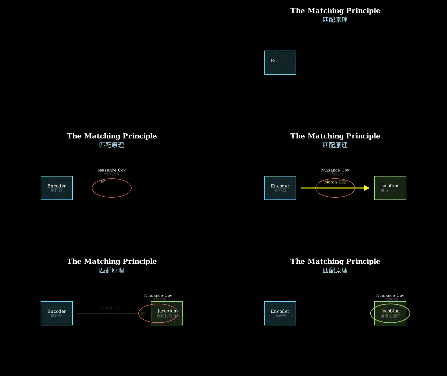
The method has three components: (1) identify which variations in deployment preserve labels (nuisance), (2) estimate their covariance structure Sigma, (3) regularize the encoder’s Jacobian J so its range covers Sigma’s range.

In the linear-Gaussian setting, the paper proves closed-form optimality: the encoder should perform “cube-root water-filling” within the matched subspace—allocate representation capacity proportional to the cube root of each nuisance eigenvalue. Outside the matched subspace, use isotropic regularization.

Input x --> Encoder f(x) --> Representation z --> Task head --> Output y
              |
              | Jacobian J = df/dx
              v
         [Regularizer]
              |
              +-- Match range(J) to range(Sigma)
              |   where Sigma = Cov(label-preserving noise)
              |
              +-- Within matched subspace: cube-root water-filling
              +-- Outside matched subspace: isotropic penalty

Think of it like designing a suspension system for a car. You don’t want the suspension to be uniformly stiff in all directions—that wastes energy dampening irrelevant vibrations. Instead, you measure which road bumps actually matter (the ones that don’t flip the car), estimate their typical magnitude and direction (the covariance Sigma), then tune each suspension spring to absorb exactly those shocks (match the range). The cube-root water-filling is like allocating stiffer springs to the directions with bigger bumps, but with diminishing returns—you don’t need a spring ten times stiffer for a bump ten times bigger, because the relationship is sublinear.

Key Concepts

• Deployment nuisance: Variations between training and deployment that don’t change the correct label. Examples: lighting changes in images (object identity unchanged), speaker accent in speech (word unchanged), writing style in text (meaning unchanged). The key insight is that these nuisances have geometric structure—they’re not arbitrary noise, but live in a subspace. A photo of a cat under different lighting traces out a manifold in pixel space; the covariance of that manifold is what we need to estimate.

• Range matching: If your encoder’s Jacobian has range that covers the nuisance covariance’s range, then small nuisance perturbations get mapped to small representation changes—the encoder is insensitive along nuisance directions. If the ranges don’t align, you’re either wasting capacity (encoding irrelevant dimensions) or vulnerable (missing important nuisance directions). The paper proves this is necessary for quadratic Jacobian penalties to work (Theorem G).

• Trajectory Deviation Index (TDI): A label-free diagnostic for when standard metrics fail. Suppose you fine-tune a language model and accuracy stays high, but the model becomes brittle in ways accuracy doesn’t capture. TDI measures how much embeddings deviate along a trajectory of nuisance variation (e.g., rephrasing the same question). High TDI means the representation is jittery under nuisance—a leading indicator of deployment fragility even when validation accuracy looks fine.

Framework Shift

Before (mainstream approach):        After (this paper):

  Problem 1: Domain adaptation          Deployment nuisance Sigma
  Method: CORAL                              |
                                             v
  Problem 2: Adversarial robustness     Estimate Sigma
  Method: PGD training                   (different estimators)
                                             |
  Problem 3: Augmentation                    v
  Method: RandAugment                   Regularize J to match
                                        range(J) ⊇ range(Sigma)
  Problem 4: Metric learning                 |
  Method: Triplet loss                       v
                                        Closed-form optimality:
  [Independent toolbox]                 cube-root water-filling

  Stack methods empirically             Principled geometry

From a toolbox of independent heuristics to a single statistical estimand with provable structure, the core shift is recognizing that robustness methods are solving the same geometric alignment problem.

Expert Assessment

Problem choice: This is a real gap. The field has been in a “collect more tricks” phase for years, and unification attempts (like IRM) have been narrow. The problem sits at a natural inflection point—enough methods exist to see patterns, but no one has named the shared structure. The framing as “estimate then match” is simple enough to be falsifiable, which is rare in robustness theory.

Method maturity: The linear-Gaussian analysis is rigorous and the closed-form results (cube-root water-filling, necessity of range coverage) are non-obvious. The extension to deep networks is more heuristic—the paper argues that global minima inherit the same range dichotomy, but the proof sketch relies on local linearization. The Trajectory Deviation Index is a clever diagnostic, though it requires choosing a nuisance trajectory, which reintroduces some arbitrariness.

Experimental integrity: Thirteen pre-registered experiments is strong—pre-registration prevents cherry-picking. Twelve passing and one failing (Office-31, with the failure mode predicted beforehand) is honest reporting. The experiments span classical ML to 7B-parameter LLMs, which tests generality. However, the “matched > isotropic > wrong-W” ordering is tested on geometry and drift, not always on downstream task performance, which is what practitioners care about. The Qwen2.5-7B alignment experiment is intriguing but small-scale.

Writing quality: The abstract is dense and assumes familiarity with the robustness zoo. The paper would benefit from a “running example” that threads through all sections—pick one concrete task (say, sentiment analysis under style shift) and show how CORAL, adversarial training, and augmentation all estimate the same Sigma for that task. The theorems are stated precisely, but the intuition often comes after the formalism, which makes the paper harder to read than necessary.

Verdict: weak accept — The unification is conceptually valuable and the linear-Gaussian theory is solid, but the deep network extension is incomplete and the experiments don’t fully close the loop to task performance. This is a strong foundation paper that will need follow-up work to become actionable at scale.

Takeaways

For practitioners: If you’re stacking robustness methods (augmentation + adversarial training + domain adaptation), you might be estimating the same nuisance covariance three times with different noise. Instead, explicitly estimate Sigma once (e.g., via augmentation or domain statistics), then regularize your encoder’s Jacobian to match it. The Trajectory Deviation Index is immediately useful—if you’re fine-tuning a model and accuracy plateaus but TDI spikes, you’re degrading robustness in ways validation loss won’t catch.

For researchers: The “estimate then match” framing is a template for unifying other method families. The cube-root water-filling result suggests that optimal robustness is sublinear in nuisance magnitude, which contradicts the “more augmentation is always better” intuition. The pre-registration protocol (predict failure modes before running experiments) should be standard practice.

For theorists: The necessity of range coverage (Theorem G) is a falsifiable constraint—if a Jacobian penalty works but doesn’t satisfy range coverage, the theory is wrong. The gap between linear-Gaussian optimality and deep network behavior is where the next theoretical work should focus.