The FID Lottery: Why Your Benchmark Number Is Luckier Than You Think

Paper: 2606.20536 Authors: Nicolas Dufour, Alexei A. Efros, Patrick Pérez Categories: cs.CV

The Gap

Existing practice treats FID as a deterministic number: train one model, pick one seed, compute one value, call it the score. A few papers report FID over multiple samples from a fixed model, but almost nobody varies the training seed. The implicit assumption is that training noise — random initialisation, data ordering, Gaussian noise in the flow-matching loss — averages out. The authors show this assumption is false.

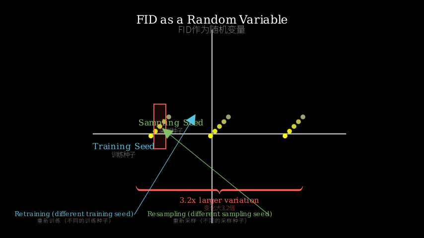
They train several hundred SiT networks on class-conditional ImageNet 256x256, systematically varying both training seeds and generation seeds. This lets them decompose FID variance into its sources and measure their relative magnitudes. The evidence is quantitative and exhaustive: retraining shifts FID 3.2x more than resampling from a fixed network.

[Problem]         +--  One FID number  --+    [Assumption]
  FID used as           published              Training noise
  ground truth                                  is negligible
       v                                        v
[Question]         +--  Treat FID as     --+  [Method]
  How much does          a random           Train 200+ models
  FID actually          variable           on two axes: train
  vary?                                     seeds + gen seeds
       v                                        v
[Evidence]         +--  Retrain variance 3.2x > sample variance
  400+ models          CoV ~1-2%           Count the sources
  on ImageNet                              (init, data order, noise)
       v                                        v
[Conclusion]
  No single FID number is reliable.
  Report error bars over training seeds.
  Gaps below ~1.3% CoV are inconclusive.

The Increment

One sentence: Before this paper, FID was treated as a trustworthy point estimate; after this paper, it is an unbounded random variable whose dominant variance component comes from retraining, not sampling.

Core Mechanism

The authors construct a two-axis experiment panel: the training axis and the generation axis. Along the training axis, they start from different random seeds (affecting weight initialisation, data-shuffle order, and the per-step Gaussian noise in the flow-matching loss). Along the generation axis, they draw different sets of 50,000 images from a fixed trained model.

For each cell in this grid — a specific (training seed, generation seed) pair — they compute a single FID. By collecting many cells, they can decompose the total variance: how much comes from the training axis, how much from the generation axis, and how much from their interaction.

The key operation is ANOVA-like variance decomposition on the FID values. They also introduce a practical trick: per-cell classifier-free guidance (CFG) tuning. Instead of using a fixed guidance scale λ for all training seeds, they optimise λ separately for each cell. This halves the spread and rescues the unluckiest seeds, but it reshuffles which seeds perform best.

[Training Seed] -> [SiT Model] -> [50k Samples] -> [FID]  <--  one cell
        ^               ^               ^
   random init      data order      Gaussian noise
   (seed)          (seed)          in loss (seed)

[Experiment Grid]      gen seed 1    gen seed 2  ...  gen seed 10
  train seed 1          FID_11        FID_12         FID_110
  train seed 2          FID_21        FID_22
  ...
  train seed 20         FID_201

[variance breakdown]  ->  total variance = var(train) + var(gen) + var(interaction)
                        ->  var(train) : var(gen) ~ 3.2 : 1

Think of this as a lottery with two tiers. The first tier (training seed) determines which lottery ticket you hold — your initialisation, your data order, your luck with the per-step Gaussian noise. The second tier (generation seed) determines which 50,000 tickets you scratch off from that ticket.

Most labs report the result of scratching one ticket from one ticket — a single FID. What this paper shows is that the prize pool is huge: holding a “lucky” training ticket can save you up to 2× compute to reach the same FID as an “unlucky” ticket. And changing the training ticket (retraining) moves the prize 3.2× more than scratching a different set of tickets from the same ticket (resampling).

The per-cell CFG tuning is like allowing each ticket holder to choose their own scratch-off technique. It halves the spread, but it also reshuffles which tickets pay out best — so you can no longer compare scores across different guidance scales.

Key Concepts

• Variance Decomposition (ANOVA-style):
  Imagine you’re measuring the height of plants in a field. The total variation comes from three sources: different seed varieties (training seed), different watering schedules (generation seed), and their interaction. ANOVA splits the total into these components. Here, the “height” is FID, and the sources are training randomness and generation randomness. The paper finds that the “seed variety” factor (training seed) is 3.2× more important than the “watering” factor (generation seed). If you only water differently (resample), you don’t see the full range.

• Coefficient of Variation (CoV):
  Standard deviation divided by mean, expressed as a percentage. If FID is 10 with a CoV of 1.5%, that means one standard deviation is 0.15 FID points. Why does this matter? If you see a paper claiming a 0.3 FID improvement over a baseline, and the CoV is 1.5%, the gap is only 2 standard deviations apart — barely significant. The authors measure CoV across models of different sizes and compute budgets, finding it stays in a 1-2% band no matter what. So a 1-2% FID gap is the noise floor.

• Classifier-Free Guidance (CFG) Tuning:
  In conditional generation, CFG trades off diversity vs. fidelity via a scale λ. Usually λ is fixed for all experiments. This paper tunes λ per training seed to minimise FID. Why? Because different training seeds produce models with slightly different optimal λ. Fixing λ penalises the unlucky seeds. After per-cell tuning, the spread halves. But the cost is apples-to-oranges comparison: two FIDs at different λ are not on the same scale.

Framework Shift

Before (mainstream approach):
  [Train one model with one seed]
         |
    [Sample one set of 50k images with one seed]
         |
    [Compute one FID number]
         |
    [Publish as "the" score]
    [Compare to other papers' single numbers]

After (this paper's approach):
  [Train 5-10 models with different seeds]
       |           |           |
  [Optimise CFG per model] [Optimise CFG per model]
       |           |           |
  [Sample 50k images per model]
       |           |           |
  [Compute mean FID + std across models]
       |           |           |
  [Report as: FID = 10.23 +/- 0.15]
  [Declare any gap < 0.20 as inconclusive]

One sentence: From treating FID as a precise number to treating it as a random draw from a distribution with a stable ~1.3% CoV, the core shift is adopting error bars over training seeds as the minimal credible unit of evaluation.

Expert Assessment

Problem choice: This is a genuine and overdue gap. The field has been using FID as a cudgel in leaderboards and paper comparisons for years, despite widespread intuition that it’s noisy. The authors turn that intuition into measurement. It sits at the intersection of reproducibility and evaluation methodology — not flashy, but foundational. Every generative-model paper from now on should cite this.

Method maturity: The approach is simple and elegant: treat FID as a random variable and measure its variance via brute-force repetition. That’s not clever; it’s correct. An even simpler approach would be to just report the variance over training seeds without the ANOVA decomposition, but the decomposition is what makes the 3.2× finding concrete. The per-cell CFG tuning is the one clever addition. Some might argue the paper is “just a measurement” — but that measurement is what was missing.

Experimental integrity: The authors train several hundred SiT models. That’s expensive but thorough. Baselines are fair because they compare against themselves (retraining vs resampling). The choice of SiT over DiT or other architectures is reasonable for compute reasons, and the class-conditional ImageNet setting is standard. One potential red flag: all experiments use the same architecture family. Would the CoV band hold for GANs or VAEs? The paper doesn’t say. But for score-based diffusion models, the evidence is solid.

Writing quality: The paper is well-structured and the findings are presented clearly. The weakest section is the discussion of *why the CoV band is so stable across model sizes and compute budgets. They show it’s true, but the explanation is thin: “three factors (init, data order, noise) are invariant to scale.” That’s plausible but not proven. A deeper analysis of where the residual variance comes from would elevate the paper from “phenomenological” to “mechanistic.”

Verdict: Strong accept — This paper fixes a blind spot that has infected hundreds of prior evaluations. It doesn’t invent a new method; it invents a new *standard for evaluation.

Takeaways

1. Report FID as a distribution over training seeds, not a point estimate.
   Even 5 seeds (with per-seed CFG tuning) give a mean and std that are far more informative than a single number.

2. Adopt a 1-2% CoV as the noise floor for diffusion models on ImageNet.
   Any claimed improvement below this threshold — especially from a single run — should be treated as inconclusive.

3. Per-seed CFG tuning is a practical cheap fix to reduce variance by ~2x.
   But don’t compare FIDs across different guidance scales; the numbers are not on the same axis.

4. The “lucky seed” compute gap is real. If you find a good training seed, you can report the same FID with half the compute. This is an incentive to cherry-pick. The fix is to pre-commit to a set of seeds and report all results.