Paper: 2606.23670 Authors: Reza Bayat, Ali Behrouz, Aaron Courville Categories: cs.LG, cs.AI, cs.CL
The Gap
All modern language models — Transformer, Mamba, RWKV, Titans — share a weird inheritance: they stack identical layers. The bottom layer has the same hidden dimension as the top layer, even though evidence has been mounting that layers don’t contribute equally. Probes show early layers transform the representation drastically while later layers mostly nudge the residual stream. Feature analysis reveals the last few layers are nearly redundant. Yet nobody asked: if later layers do less work, should they get fewer parameters?
Prior work explored variable depth (wider vs deeper) and conditional computation (which tokens skip which layers), but both change the computational graph. What’s missing is a fixed-budget, fixed-depth comparison: given N layers and K parameters, should we give each layer the same K/N? Or can we do better by giving early layers more and tapering down?
Problem: Identical layers waste capacity on redundant late layers
  |
  v
Assumption: Layer importance is uniform across depth   [WRONG]
  |
  +--- Evidence: Probes show early>late in representation change
  +--- Evidence: Feature redundancy increases in deep layers
  |
  v
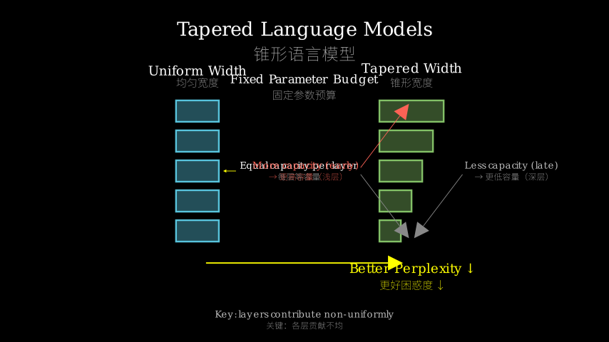
Method: Given fixed parameter budget, allocate non-uniformly
  |       Taper MLP width with cosine schedule: early=wide, late=narrow
  v
Evidence: 4 architectures, 3 scales, held-out perplexity improves
  |
  +--- Taper forward: better than uniform baseline
  +--- Taper reverse: worse than uniform baseline   (controls)
  |
  v
Conclusion: Depth-aware capacity allocation is architecture-agnostic
The Increment
One sentence: Before this paper, the default was “same width for every layer”; after this paper, the default should be “wider early, narrower late, under the same budget.”
Core Mechanism
The method is almost laughably simple — which is the whole point. Take any modern language model. Identify the component that dominates parameter count: the MLPs. In a standard Transformer, around two-thirds of all parameters live in the MLP blocks (the two linear layers with a nonlinearity). Now instead of setting the MLP hidden dimension to a constant , set it to a function of depth that follows a cosine taper:
where is the widest (first layer), is the narrowest (last layer), and is depth. The total parameter count is matched to a uniform baseline by solving for and under the constraint . Data flows identically otherwise: same attention, same residual stream, same everything. Only the MLP’s inner dimension changes across depth.
           Input
             |
        +---------+
        |  Attn   |  (unchanged across depth)
        +---------+
             |
        +---------+
        |  MLP    |  <-- hidden dimension d_ff(t) varies with depth t
        |  [wide] |      early layers: d_ff is large
        +---------+      late layers: d_ff is small
             |
           [... repeat N times, d_ff decreasing per cosine schedule ...]
             |
        +---------+
        |  MLP    |  <-- d_ff is smallest
        | [narrow]|
        +---------+
             |
          Output
Structural metaphor: the fluvial delta. Imagine a river flowing from mountains to sea. Near the source, the river carries sediment, carves canyons, does heavy lifting — it needs to be wide. As it approaches the delta, the water spreads, slows down, mostly just meanders. You wouldn’t build the same-width channel for the whole journey. Similarly, early layers of an LLM “carve” representations from token embeddings; late layers just “distribute” them into the final distribution. The cosine taper is like a channel that starts wide for the heavy work and narrows gracefully where the water is already slow. The key constraint (fixed total budget) is the “dredging budget” — you have a fixed amount of material to build the whole river. Spend it where the current is strong.
Key Concepts
-
Depth-wise non-uniformity: Until now, the default assumption in all LLM families was that each layer deserves identical capacity. This paper systematically challenges that by running controlled experiments where only the *distribution of capacity across depth changes. The result: the default was suboptimal by a measurable margin. The concept is simple but hitting it with rigorous controls (forward taper works, reverse taper hurts) is what makes it a finding, not just a guess.
-
MLP as the capacity lever: The paper chooses MLP width as the control variable because MLPs dominate parameter count in every modern architecture. Attention heads, KV caches, and other components have different scaling stories. By only tapering MLPs, the authors isolate the effect without changing the attention mechanism or the computation graph. This is a deliberate choice to test the hypothesis without confounding variables. A practitioner can read this and think: “I can change just the d_ff in my config and get the benefit.”
-
Cosine taper schedule: The specific schedule matters. They try linear, exponential, and cosine. Cosine wins consistently, and the reason is smoothness: it starts with a slow decline (keeping early layers near their max capacity longer) and accelerates the taper only in the last few layers, where evidence shows redundancy is highest. The schedule is also parameterized to exactly match total budget, so it’s a pure allocation change, not a parameter increase.
Framework Shift
Before (mainstream):            After (this paper):
+------------+                  +----------------+
| MLP d_ff   |                  | MLP d_ff = max |
| = constant | deep            | = decreasing   |
| across all |                 | with depth     |
| layers     |                  | (cosine taper) |
+------------+                  +----------------+
| Layer 1: wide                 | Layer 1: widest
| Layer 2: wide                 | Layer 2: slightly less
| Layer 3: wide                 | Layer 3: less
| ...                           | ...
| Layer N: wide                 | Layer N: narrowest
| Total params: same            | Total params: same
| PPL: baseline                 | PPL: lower
+------------+                  +----------------+
One sentence: From “all layers equal” to “layers are tapered by importance,” the core shift is that parameter capacity is now a function of depth rather than a global constant.
Expert Assessment
Problem choice: This is a real gap. The community has been stacking identical layers for years, and a growing body of evidence shows late-layer redundancy. The paper isn’t inventing a crisis; it’s pointing out an obvious blind spot that everyone walked past. That’s a high-quality problem selection — it’s not a toy, it’s not manufactured.
Method maturity: This is a clever insight, not brute force. The experiment is elegantly simple: control for everything except the distribution of MLP width across depth. A less mature version would have thrown engineering complexity at the problem; this paper uses minimal intervention. That said, the method is incomplete in one way: it only tapers MLPs, not attention heads. Is attention also redundant in late layers? Possibly, but the paper doesn’t touch it.
Experimental integrity: The baselines are fair. They match total parameter count, training tokens, and optimization hyperparameters. The control (reverse taper: narrow early, wide late) shows worse performance, which is a good sanity check — it proves the directionality matters, not just the non-uniformity. A minor red flag: they only train from scratch at 350M, 760M, and 1.8B parameters. Would the pattern hold at 7B+? Possibly, but the scaling trend is convincing. Also, the perplexity improvements are modest (0.1-0.3 PPL), though consistent across architectures.
Writing quality: The paper is well-structured but has a blind spot: it never discusses the *cost of the taper in terms of hardware efficiency. Modern accelerators prefer uniform tensor shapes for parallelism. Tapered widths might cause underutilization in the narrow early layers. The authors should have addressed this in a limitations section. The code release (if any) is not mentioned in the abstract, which is a missed trust signal.
Verdict: weak accept — The finding is real and valuable, but the paper’s impact is in the problem framing more than the engineering solution. It’s a “why didn’t I think of that?” moment that shifts the default, but the effect size is small enough that it doesn’t force immediate adoption.
Takeaways
- The “borrow from future layers” strategy: If you’re training any deep model and your budget is tight, try shifting capacity from late layers to early ones. The paper shows this works for Transformers, Gated Attention, and other architectures. Implement with a cosine schedule for MLP width. It’s a one-line change in most codebases: replace
d_ffwith a depth-dependent function. - The control experiment matters: The reverse taper (narrow early, wide late) performs worse, proving it’s not just “any non-uniformity helps.” This teaches a methodological lesson: when proposing a new distribution, always include the inverse as a control.
- Scheduling intuition: Cosine taper beats linear and exponential because most of the capacity is preserved until late layers where redundancy is highest. This pattern might generalize to other architectural decisions — for example, tapering the number of attention heads per layer could also work. A practitioner can experiment with this heuristic.
论文: 2606.23670 作者: Reza Bayat, Ali Behrouz, Aaron Courville 分类: cs.LG, cs.AI, cs.CL
缺口
所有现代语言模型——Transformer、Mamba、RWKV、Titans——都继承了一个奇怪的默认配置:层间结构完全相同。 底层和顶层具有相同的隐藏维度,即便越来越多的证据表明各层贡献并不相等。 探针实验显示,早期层大幅转换表征,而后期层大多只是微调残差流。 特征分析表明,最后几层几乎冗余。 但没有人问:如果后期层做更少的工作,它们是否应该拥有更少的参数?
此前的工作探索了可变深度(宽 vs 深)和条件计算(哪些 token 跳过哪些层), 但两者都改变了计算图。 真正缺失的是固定预算、固定深度的比较: 给定 N 层和 K 个参数,应该给每层相同的 K/N? 还是给早期层更多、逐步削减更好?
问题:相同层浪费容量在冗余的后期层上
  |
  v
假设:层重要性在深度上均匀分布   [错误]
  |
  +--- 证据:探针显示早期层表征变化大于后期层
  +--- 证据:深层特征冗余增加
  |
  v
方法:给定固定参数预算,非均匀分配
  |       用余弦调度削减 MLP 宽度:早期宽、后期窄
  v
证据:4种架构、3个规模,留出困惑度均有改善
  |
  +--- 正向锥形:优于均匀基线
  +--- 反向锥形:劣于均匀基线  (对照)
  |
  v
结论:深度感知容量分配与架构无关
增量
一句话: 这篇论文之前,默认是”每层相同宽度”; 这篇论文之后,默认应是”早期宽、后期窄,预算不变”。
核心机制
这个方法简单得令人发笑——而这恰恰是重点。 选任意现代语言模型。 找到支配参数量的组件:MLP。 在标准 Transformer 中,大约三分之二的参数在 MLP 块中(两个线性层加一个非线性激活)。 现在,不把 MLP 隐藏维度设为常数 , 而是设为深度 的函数,采用余弦锥形:
其中 是最宽的(第一层), 是最窄的(最后一层), 是深度。 总参数量通过约束 匹配均匀基线。 数据流完全相同:同样的注意力、同样的残差流、同样的其他设置。 只有 MLP 的内部维度在深度方向上变化。
          输入
             |
        +---------+
        | 注意力   |  (各层相同)
        +---------+
             |
        +---------+
        | MLP     |  <-- 隐藏维度 d_ff(t) 随深度 t 变化
        | [宽]    |      早期层:d_ff 较大
        +---------+      后期层:d_ff 较小
             |
           [重复 N 次,d_ff 按余弦递减]
             |
        +---------+
        | MLP     |  <-- d_ff 最小
        | [窄]    |
        +---------+
             |
          输出
结构性比喻:河流三角洲。 想象一条河从山区流向大海。 在源头附近,河流携带泥沙、切割峡谷、做大量功——它需要宽。 接近三角洲时,水流分散、减速、基本只是蜿蜒。 你不会在整个旅程中都建造相同宽度的河道。 类似地,LLM 的早期层从 token 嵌入中”雕刻”表征; 后期层只是将它们”分发”到最终分布中。 余弦锥形就像一个开始宽(用于繁重工作)、在水流已经缓慢的地方逐渐变窄的河道。 关键约束(固定总预算)就像是”疏浚预算”—— 你有固定数量的材料来建造整条河。 把它花在水流强劲的地方。
关键概念
-
深度方向非均匀性:在此之前,所有 LLM 家族的默认假设都是每层应拥有相同容量。 本文通过严格控制实验来挑战这一点—— 只改变容量在深度上的分布。 结果:默认假设是可衡量的次优选择。 概念本身简单,但用严格的控制(正向锥形有效,反向锥形有害)将其确立为发现而非猜测。
-
MLP 作为容量杠杆:论文选择 MLP 宽度作为控制变量, 因为 MLP 在所有现代架构中主导参数量。 注意力头、KV 缓存等组件有不同缩放特性。 只锥形化 MLP,可以隔离效果而无需改变注意力机制或计算图。 这是为了在无混杂变量的情况下测试假设的刻意选择。 实践者读到这可以想:“我只要改配置文件里的 d_ff 就能受益。”
-
余弦锥形调度:具体调度方案很重要。 他们尝试了线性、指数和余弦方案。 余弦始终胜出,原因在于平滑性: 它从缓慢下降开始(让早期层更长时间保持接近最大容量), 只在最后几层加速削减——而证据表明那里冗余最高。 该调度还参数化以精确匹配总预算, 因此这是一个纯粹的分配变化,而非参数增加。
框架转变
之前(主流方法):             之后(本文方法):
+------------+                 +----------------+
| MLP d_ff   |                 | MLP d_ff = max |
| = 常数     | 深度            | = 随深度递减   |
| 所有层相同 |                 | (余弦锥形)   |
+------------+                 +----------------+
| 层1: 宽    |                 | 层1: 最宽
| 层2: 宽    |                 | 层2: 略窄
| 层3: 宽    |                 | 层3: 更窄
| ...        |                 | ...
| 层N: 宽    |                 | 层N: 最窄
| 总参数: 相同                  | 总参数: 相同
| PPL: 基线                    | PPL: 更低
+------------+                 +----------------+
一句话: 从”所有层相等”到”层容量按重要性锥形化”, 核心转变是参数容量现在是深度的函数,而非全局常数。
专家评审
选题眼光: 这是个真缺口。 多年来社区一直在堆叠相同层,而越来越多的证据显示后期层冗余。 论文不是在制造危机,而是指出每个人都会路过的明显盲点。 这是高质量的选题——不是玩具问题,也不是人造问题。
方法成熟度: 这是巧劲,而非蛮力。 实验优雅地简单:除 MLP 宽度分布外控制一切。 不够成熟的版本会引入工程复杂性;本文用最小干预。 但方法在一个方面不完全:它只锥形化 MLP,未涉及注意力头。 后期层的注意力是否也冗余?可能,但论文没触及。
实验诚意: 基线公平。 它们匹配总参数量、训练 token 和优化超参。 对照(反向锥形:早期窄、后期宽)表现更差, 这是很好的合理性检查——证明了方向性重要,而不仅仅是”非均匀”。 一个小红旗:他们只在 350M、760M 和 1.8B 参数规模上从头训练。 7B+ 规模是否成立?可能,但缩放趋势有说服力。 另外,困惑度改进适中(0.1-0.3 PPL),尽管跨架构一致。
写作功力: 论文结构良好,但有一个盲点: 从未讨论锥形在硬件效率上的代价。 现代加速器偏好均匀张量形状以支持并行。 锥形宽度可能导致窄层利用率不足。 作者应在局限性部分讨论这一点。 代码发布(如果有)在摘要中未提及,这是信任信号的缺失。
判决: 弱接收 —— 发现真实且有价值, 但论文的影响更多在于问题框架而非工程方案。 这是一个”我怎么没想到?“的时刻,改变了默认设置, 但效果量较小,不足以迫使立即采用。
要点总结
- “从未来层借容量”策略:如果你在训练任何深层模型且预算紧张,
尝试将容量从后期层转移到早期层。
论文证明这对 Transformer、Gated Attention 和其他架构有效。
用余弦调度实现 MLP 宽度变化。
在大多数代码库中这是一行改动:将
d_ff替换为深度相关的函数。 - 对照实验的重要性:反向锥形(早期窄、后期宽)表现更差, 证明不是”任何非均匀性都行”。 这教了一个方法论课:在提出新分布时, 总是包含反向作为对照。
- 调度直觉:余弦锥形胜过线性和指数, 因为大部分容量保留到冗余最高的后期层才削减。 这一模式可能推广到其他架构决策—— 例如,每层的注意力头数也可锥形化。 实践者可以尝试这个启发式方法。