Stop Probing, Start Coding: Why Sparse Autoencoders Fail at Compositional Generalization

Paper: 2603.28744 Authors: Vitória Barin Pacela, Shruti Joshi, Isabela Camacho, Simon Lacoste-Julien, David Klindt Categories: cs.LG

The Gap

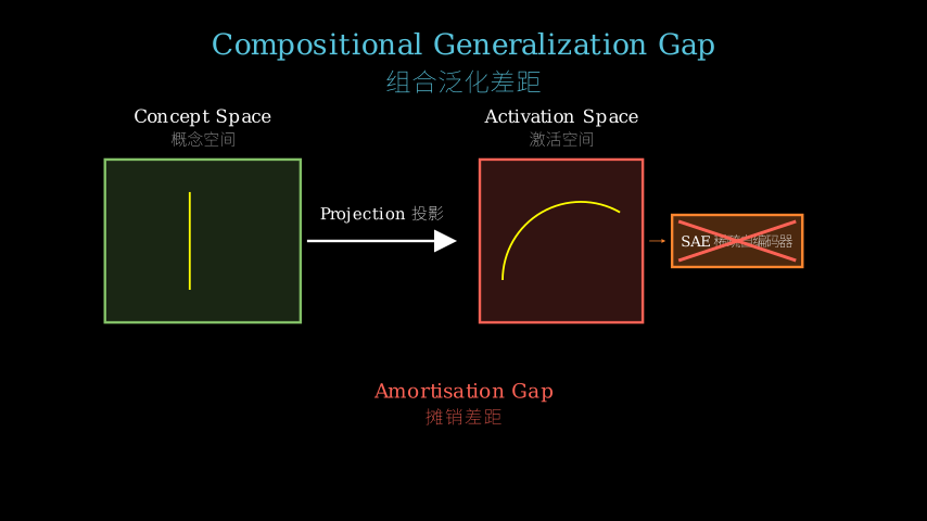
Linear probes and sparse autoencoders (SAEs) are the go-to tools for interpreting neural network representations. The linear representation hypothesis says high-level concepts live as linear mixtures in activation space. SAEs try to unmix these by learning sparse dictionaries. They work fine on in-distribution data, but collapse under compositional shifts—new combinations of known concepts.

The field assumed this was an amortization problem: SAEs use a fixed encoder instead of per-sample iterative inference like FISTA. But no one had cleanly separated dictionary quality from inference quality. This paper does that decomposition and finds the opposite: the dictionaries themselves are broken.

Problem: SAEs fail on OOD compositional shifts
    |
    v
Assumption: Amortization gap (fixed encoder vs iterative)
    |
    v
Method: Swap SAE encoder with FISTA on same dictionary
    |
    v
Evidence: Gap persists -> dictionary is wrong, not encoder
    |
    v
Conclusion: Dictionary learning is the bottleneck

The Increment

One sentence: Before this paper, we blamed SAE failures on amortized inference; after, we know the learned dictionaries point in wrong directions and that’s the real problem.

Core Mechanism

The method is a controlled ablation. Start with a trained SAE (dictionary + encoder). The SAE encoder is amortized—it’s a fixed neural network that maps activations to sparse codes in one shot. Classical sparse coding uses iterative algorithms like FISTA that solve an optimization problem per sample, which should recover better codes if the dictionary is good.

The experiment: freeze the SAE’s dictionary, throw away its encoder, and replace it with FISTA. If the amortization gap hypothesis is right, FISTA should close the gap. If the dictionary hypothesis is right, FISTA will still fail because it’s optimizing over a bad dictionary.

SAE Pipeline:
activation -> [encoder NN] -> sparse code -> [dictionary] -> reconstruction
                (amortized)                      (learned)

Ablation Pipeline:
activation -> [FISTA solver] -> sparse code -> [same dictionary] -> reconstruction
                (iterative)                       (from SAE)

Oracle Baseline:
activation -> [FISTA solver] -> sparse code -> [true dictionary] -> reconstruction
                (iterative)                       (ground truth)

Think of it like a treasure map. The dictionary is the map itself—it tells you which directions to search. The encoder is your navigation strategy—either you follow a pre-planned route (amortized) or you adjust step-by-step based on terrain (iterative). If the map has wrong landmarks, even the best navigation won’t find the treasure. This paper shows SAEs draw maps with landmarks in wrong places. Swapping navigation strategies doesn’t help because you’re still following a bad map. The oracle baseline proves that with the correct map, even simple navigation works.

Key Concepts

• Superposition: Neural networks pack more concepts than they have dimensions. Imagine a 3D room storing 10 different objects by overlapping their shadows on the walls. Each wall (dimension) shows a mixture of multiple objects (concepts). To recover which objects are present, you need to unmix the shadows. This is hard because the projection loses information—different object combinations can cast similar shadows.

• Amortization Gap: Classical sparse coding solves an optimization problem for each input: “find the sparsest code that reconstructs this activation well.” This is slow but accurate. SAEs train a neural network to predict the answer directly, trading accuracy for speed. The gap is the performance difference. Everyone assumed this gap explained SAE failures, but this paper shows it doesn’t.

• Dictionary Learning: The dictionary is a matrix where each column represents a “concept direction” in activation space. If concepts are “cat,” “dog,” “running,” the dictionary should have columns pointing toward pure “cat-ness,” pure “dog-ness,” etc. Learning this dictionary from data is hard because you only observe mixtures, never pure concepts. SAEs learn dictionaries that point in approximately right directions for training data but wrong directions for new combinations.

Framework Shift

Before (mainstream view):               After (this paper):

Activation                              Activation
    |                                       |
    v                                       v
[Amortized Encoder] <-- problem here   [Dictionary] <-- problem here
    |                                       |
    v                                       v
Sparse Code                             Sparse Code
    |                                       |
    v                                       v
[Dictionary]                            [Inference Method]
    |                                       |
    v                                       v
Reconstruction                          Reconstruction

Fix: Use iterative inference           Fix: Learn better dictionaries

From blaming the inference shortcut to blaming the learned geometry, the core shift is recognizing that fast approximation isn’t the bottleneck—wrong directions are.

Expert Assessment

Problem choice: Real gap. Interpretability tools failing on distribution shifts is a practical blocker, not a manufactured concern. The compositional generalization angle is well-motivated—if SAEs can’t handle new combinations of known concepts, they’re not really disentangling concepts.

Method maturity: Elegant decomposition. The ablation design is simple but decisive: swap one component, hold everything else fixed, measure. The oracle baseline is crucial—it proves the problem is solvable at the scales tested, so this isn’t a fundamental limitation. No obvious simpler approach was overlooked.

Experimental integrity: Baselines are fair. The controlled synthetic experiments isolate the failure mode cleanly. The progression from toy problems to realistic scales is convincing. One minor concern: the “true dictionary” oracle assumes you know ground truth concept directions, which you never have in real interpretability work. But for a diagnostic paper, this is acceptable.

Writing quality: The abstract and intro are sharp. The related work section is dense—could be trimmed. The experimental section is thorough but repetitive across scales. The discussion could push harder on what “scalable dictionary learning” actually means in practice. Rewriting Section 4.3 to propose concrete next steps would elevate the paper from diagnostic to actionable.

Verdict: strong accept — Clean experimental design that overturns a widely-held assumption and reframes a practical problem with clear implications for future work.

Takeaways

If you’re building sparse coding systems, don’t throw compute at amortization. Invest in dictionary initialization and learning objectives. The paper suggests classical sparse coding theory (compressed sensing, incoherence conditions) might guide better dictionary learning, but that’s underexplored in the deep learning era.

For interpretability practitioners: SAE-extracted “features” are less reliable under distribution shift than you think. If you’re using them for safety-critical applications, test compositional robustness explicitly.

The broader lesson: when a learned system fails, decompose it. Don’t assume the obvious bottleneck (here, amortization) is the real one. Ablate components systematically.