Spectrally-Guided Diffusion Noise Schedules: Tailoring Noise to Image Frequency Content

Paper: 2603.19222 Authors: Carlos Esteves, Ameesh Makadia Categories: cs.CV, cs.LG

The Gap

Diffusion models use noise schedules—the sequence of noise levels during training and sampling—that are handcrafted and resolution-dependent. A schedule tuned for 256×256 images breaks when you move to 512×512. Worse, the same schedule applies to all images regardless of their content: a smooth gradient gets the same treatment as a detailed texture. This one-size-fits-all approach wastes computation on redundant denoising steps and limits quality in fast sampling regimes (10-20 steps).

Prior work (DDPM, DDIM, EDM) treats noise scheduling as hyperparameter tuning—try different curves, pick what works. No one asks: what does this specific image need?

Problem: Universal noise schedules waste steps
    |
    v
Observation: Images have different spectral content
    |
    v
Method: Derive noise bounds from frequency analysis
    |
    v
Evidence: Tighter schedules improve quality at low steps
    |
    v
Conclusion: Per-instance scheduling beats fixed schedules

The Increment

One sentence: Before—all images follow the same noise schedule; after—each image gets a custom schedule based on its frequency content.

Core Mechanism

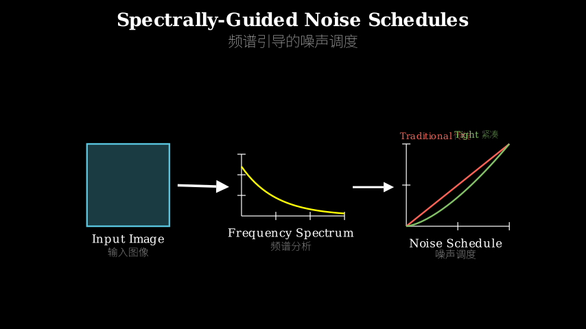
The method analyzes an image’s frequency spectrum to determine the minimum and maximum noise levels needed. High-frequency images (lots of detail) need less maximum noise because their structure is already complex. Low-frequency images (smooth regions) can skip early denoising steps because there’s nothing fine-grained to recover yet.

The authors derive theoretical bounds: minimum noise must preserve signal above the noise floor, maximum noise must not destroy recoverable frequency components. For a given image, compute its power spectral density, find where signal energy concentrates, and set noise bounds accordingly. During training, sample noise levels within these bounds. During inference, predict the image’s spectral properties from intermediate denoising states and adjust the schedule on-the-fly.

Image --> FFT --> Power Spectrum
            |
            v
    Frequency Analysis
            |
            +---> Min Noise (signal floor)
            |
            +---> Max Noise (detail ceiling)
            |
            v
    Tight Schedule [t_min ... t_max]
            |
            v
    Diffusion Process (fewer redundant steps)

Think of it like tuning a radio. A fixed noise schedule is like always scanning from 0 to 100 MHz regardless of what station you want. This paper says: if you’re looking for FM radio (high frequency content), start at 88 MHz. If you want AM (low frequency), scan 0.5-1.6 MHz. The spectral analysis is your frequency guide—it tells you where the signal actually lives, so you don’t waste time scanning empty bands. The “tight schedule” is the optimized scan range. Each image is a different station, so each gets its own range.

Key Concepts

• Spectral Properties: An image’s frequency content—how much energy sits in low frequencies (smooth gradients, large shapes) versus high frequencies (edges, textures, fine details). You can visualize this by taking the Fourier transform: a photo of a clear sky has energy concentrated in low frequencies, while a photo of tree bark spreads energy across high frequencies. The key insight: if an image has no high-frequency content, you don’t need to denoise at fine-grained noise levels—there’s nothing there to recover.

• Noise Schedule Tightness: Traditional schedules span a wide range of noise levels (say, 0.001 to 0.999) to handle all possible images. A “tight” schedule narrows this range based on what the specific image needs. If your image’s highest frequency component is at 50% of the Nyquist limit, you can cap maximum noise at a lower level—anything beyond that just destroys information you don’t have. Similarly, if there’s no ultra-fine detail, you can skip the lowest noise levels. Tightness = eliminating provably useless steps.

• Per-Instance Scheduling: Instead of one schedule for all images, generate a custom schedule for each image during inference. The model predicts spectral properties from partially denoised images (you can estimate frequency content even from noisy versions), then adjusts remaining denoising steps accordingly. It’s like adaptive bitrate streaming—the schedule adapts to the content’s complexity in real-time.

Framework Shift

Before (fixed schedule):              After (spectral-guided):

All Images                            Each Image
    |                                     |
    v                                     v
[0.001 ======== 0.999]               Analyze Spectrum
    |                                     |
    v                                     +---> Low freq: [0.1 == 0.7]
Denoise 1000 steps                        |
                                          +---> High freq: [0.01 = 0.9]
                                          |
                                          v
                                     Denoise ~200 steps

From universal noise curves to content-aware noise bounds, the core shift is treating the schedule as a function of image statistics rather than a global hyperparameter.

Expert Assessment

Problem choice: Real gap. Fast sampling (10-50 steps) is where diffusion models struggle most, and schedule inefficiency is a known bottleneck. The observation that spectral content should inform scheduling is obvious in hindsight but genuinely unexplored. Sits at the intersection of signal processing fundamentals and modern generative models—good positioning.

Method maturity: Elegant. The theoretical derivation of noise bounds from spectral analysis is principled, not heuristic. However, the inference-time prediction of spectral properties feels like the weak link—they don’t deeply explore how accurate these predictions need to be or what happens when they’re wrong. The method is simple enough to implement but requires FFT computations that add overhead.

Experimental integrity: Baselines are fair (DDPM, EDM schedules), but the paper focuses heavily on low-step regimes where their method shines. I’d want to see more analysis at 100+ steps to verify there’s no quality degradation. The ablations are solid—they isolate the contribution of min/max bounds separately. One red flag: results are mostly on single-stage pixel diffusion, not latent diffusion models (Stable Diffusion, etc.), which limits immediate applicability.

Writing quality: The spectral analysis section is dense—they could add more visual intuition (show example spectra and corresponding schedules). The related work undersells how different this is from prior adaptive scheduling attempts. The conclusion is too brief given the conceptual shift they’re proposing.

Verdict: weak accept — Solid theoretical contribution with practical benefits in an important regime, but limited scope (pixel diffusion only) and incomplete exploration of failure modes prevent strong acceptance.

Takeaways

Practitioners can steal the core insight: analyze your data’s frequency content to set training hyperparameters. This applies beyond diffusion—any iterative refinement process (super-resolution, deblurring, neural rendering) could benefit from content-aware iteration budgets. Specifically: (1) Use FFT to profile your dataset’s spectral distribution before setting noise/iteration ranges. (2) For fast inference, predict content complexity early and allocate compute accordingly—don’t spend equal effort on simple and complex samples. (3) The “tight bounds” framing is useful: identify provably useless computation and eliminate it via analysis, not just empirical tuning.