Paper: 2603.17969 Authors: Sadık Bera Yüksel, Derya Aksaray Categories: cs.RO, cs.AI
The Gap
Robotics foundation models (think RT-2, OpenVLA, and theirkin) are impressive generalists. You give them a natural language instruction and they produce actions. But they’re trained to be statistically plausible, not formally correct. There’s no mechanism inside them that says “you must visit zone A before zone B, and never enter zone C after time step10.” They might do it by luck. They might not.
Prior work on safe robot control mostly lives in two camps. The first camp is formal methods — temporal logic planers, model predictive control with constraints, barrier functions. These work beautifully when you have a hand-crafted model of the world, but they don’t plug into a neural foundation model that speaks in latent embedings. The second camp is RLHF-style finetuning or constrained RL — you can nudge a model toward safer behavior, but you’re retraining, which is expensive, britle, and requires you to anticipate every spec at training time.
The gap: nobody had a clean way to take a frozen, pretrained robotics foundation model and enforce rich, time-dependent formal specifications at inference time without touching the weights.
Problem: Foundation models lack formal temporal guarantees
    |
    v
Assumption: Forward dynamics can be approximated over a finite horizon
    |
    v
Method: At each step, solve a constrained optimization over the action
        distribution to find the minimal perturbation satisfying STL
    |
    v
Evidence: Simulation across multiple envs + complex STL specs
    |
    v
Conclusion: Hard STL constraints can be enforced at runtime
             without retraining the base model
The Increment
One sentence: Before this paper, you had to choose between a capable foundation model and formal safety guarantees — after it, you can have both, at inference time, with no retraining.
Core Mechanism
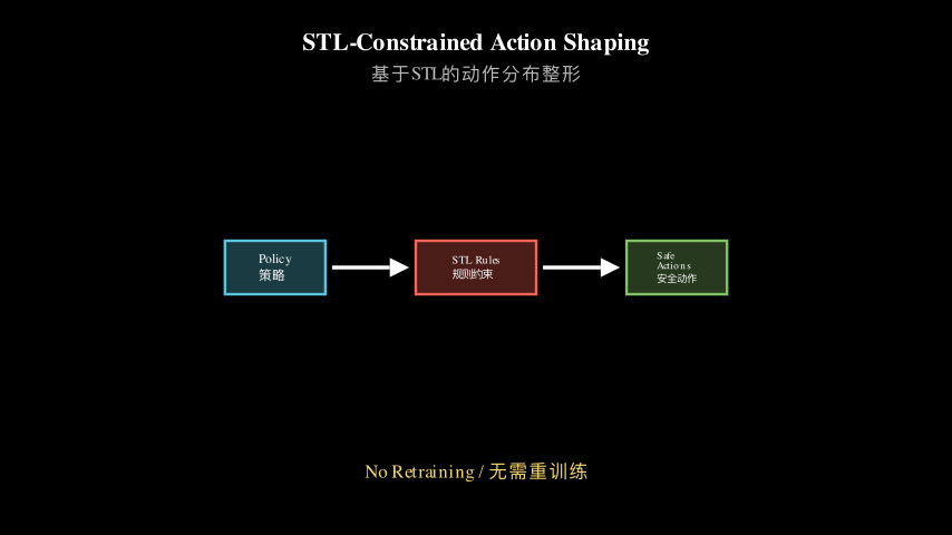
The framework sits as a thin layer on top of a pretrained robotics foundation model. At each timestep, the base model produces its usual action distribution — a probability distribution over possible next actions. Instead of sampling directly from this, the framework intercepts it.
The key operation is a constrained optimization. The framework takes the current state, the remaining time horizon, and the STL specification. It rolls out the forward dynamics — essentially simulating “if I take actions drawn from this distribution, where do I end up?” — over the remaining horizon. It then checks whether the STL formula is satisfiable given those projected trajectories. If the base model’s distribution already satisfies the constraint, great sample from it. If not, find the closest distribution (in KL-divergence or similar sense) that does satisfy the STL feasibility constraint, and sample from that instead.
The STL feasibility constraint is the hard part. STL (Signal Temporal Logic) lets you write specs like “reach goal A within10 steps, then reach goal B within 20 steps, and never enter the obstacle region.” The framework converts this into a constraint on the action distribution by propagating the dynamics forward and checking the robustness value of the STL formula — a real-valued measure of how well a trajectory satisfies the spec. The optimization finds the minimal distribution shift that keeps this robustness non-negative.
Base Model
    |
    v
[Action Distribution p(a|s,lang)]
    |
    v
+----------------------------------------+
| Specification-Aware Optimizer             |
|                                           |
|  STL spec + current state + horizon       |
|                                    |
|      v                                    |
|  Forward dynamics rollout                |
|  (simulate trajectories under p)          |
|                                    |
|      v                                    |
|  STL robustness check                     |
|  feasible? --yes-> pass through p        |
|      |                                    |
|      no                   |
|      v                    |
|  Solve: min KL(q||p) s.t. STL(q) >= 0    |
|      |                                    |
|      v                                    |
|  Modified distribution q*(a|s)            |
+------------------------------------------+
    |
    v
Sample action -> execute
Think of it like a GPS with a co-pilot. The foundation model is your driver — experienced, capable, handles most situations. The STL optimizer is the co-pilot with a rulebook. Most of the time the co-pilot says nothing and the driver does their thing. But when the driver is about to miss a required checkpoint or wander into a restricted zone, the co-pilot doesn’t grab the wheel and drive for them — they nudge the steering just enough to stay on the legal route. The driver’s style is preserved; only the trajectory is corrected. The rulebook (STL) is expressive enough to say things like “you must pass checkpoint A before checkpoint B, and you can never enter the school zone between8am and 3pm.” The co-pilot reasons ahead — “if we keep going this way, we’ll miss checkpoint A” — and adjusts early, not at the last second.
Key Concepts
-
Signal Temporal Logic (STL): A formal language for writing time-dependent rules over continuous signals. Instead of just “avoid obstacles,” you can say “reach the goal within 15 seconds AND always stay 0.5m from walls AND if you enter zone X, leave within 3 seconds.” Each formula has a robustness value — a real number that tells you not just whether the rule is satisfied, but by how much. Positive robustness = satisfied with margin. Zero = barely satisfied. Negative = violated. This real-valued property is what makes STL amenable to gradient-based optimization.
-
Distribution shaping vs. action filtering: A naive safe approach would be to just reject any action that looks unsafe and resample. That’s action filtering — it’s myopic (only looks one step ahead) and can get stuck. Distribution shaping is different: you modify the entire probability distribution over actions so that the expected future trajectory satisfies the spec. It’s proactive rather than reactive, and it reasons over the full remaining horizon.
-
Forward dynamics propagation: To check whether a distribution satisfies an STL spec, you need to know where the robot will end up. The framework uses the robot’s dynamics model to simulate forward — “if I sample actions from this distribution for the next N steps, what’s the distribution over future states?” This is the bridge between the action space and the temporal logic constraint. The quality of this propagation is a key assumption: if your dynamics model is wrong, your STL satisfaction guarantees weaken.
Framework Shift
Before (mainstream approach):        After (this paper):

  Train model with safety in mind      Pretrain model freely
         |                                    |
         v                                    v
  Hope specs are covered by data       Freeze model weights
         |                                    |
         v                                    v
  Deploy, cross fingers                At runtime: intercept
         |                             action distribution
  OR                                          |
         v                                    v
  Retrain with constrained RL          Solve STL-constrained
  (expensive, spec must be known       optimization over
   at train time)                      distribution
         |                                |
         v                                    v
  New spec? Retrain again.             New spec? Just swap
                       the STL formula.
                              |
                                              v
                       Execute with guarantees
From reactivetraining to runtime constraint injection, the core shift is: specs become a runtime parameter, not a training-time commitment.
Expert Assessment
Problem choice: This is a real gap, not a manufactured one. The tension between neural foundation models and formal guarantees is one of the central unsolved problems in robot learning right now. The paper is well-positioned — it’s not trying to solve all of safeRL, just the specific slice of “I have a frozen model, I have a spec, make it work.” That’s a tractable and practically relevant framing.
Method maturity: The core idea — constrained optimization over the action distribution at inference time — is clean and principled. It’s not brute force. The use of STL robustness as a differentiable constraint is a well-established trick borrowed from the formal methods community, and the authors apply it sensibly. That said, the forward dynamics propagation is a significant assumption. If the dynamics model is approximate (which it always is in practice), the guarantees degrade. The paper could be more upfront about how sensitive the method is to dynamics model error.
Experimental integrity: Simulation-only is the obvious limitation, and the authors acknowledge it. The choice of environments and STL specs seems reasonable for a first paper, but the baselines are thin — it’s mostly “base model without our wrapper” rather than comparison against other runtime safety methods (e.g., control barrier functions, shield synthesis). That makes it hard to know if this is the best way to solve the problem or just a working way.
Writing quality: The related work section is where the paper loses most altitude. It lists prior work without clearly articulating why each approach fails on this specific problem. A reader unfamiliar with the STL literature will struggle to understand why you can’t just use a CBF here. Rewriting that section with sharper contrast would make the contribution feel more inevitable and less incremental.
Verdict: weak accept — solid idea with clean execution, but the experimental comparison is too thin to fully trust the claims, and the dynamics model sensitivity deserves more honest treatment.
Takeaways
The most transferable idea here is the “distribution shaping as a runtime constraint layer” pattern. If you’re working with any pretrained generative model that needs to satisfy hard constraints at deployment time — not just robotics, but code generation with correctness specs, or language models with regulatory constraints — this framing is worth stealing. The specific machinery (STL robustness + KL-constrained optimization) is modular enough to swap in different constraint languages.
The second concrete takeaway: STL robustness as a differentiable objective is underused outside the formal methods community. If you have time-dependent constraints in any sequential decision problem, expressing them as STL and using the robustness value as a loss term or constraint is a practical technique that doesn’t require deep expertise in formal verification.
One honest caveat: the dynamics propagation assumption is load-bearing. Before applying this in a new domain, ask yourself how good your forward model is. If it’s poor, the “hard guarantees” soften into “soft suggestions,” and you’d be better off with a simpler approach.
论文: 2603.17969 作者: Sadık Bera Yüksel, Derya Aksaray 分类: cs.RO, cs.AI
缺口
机器人基础模型(RT-2、OpenVLA 这类)是强大的通才。 给它一条自然语言指令,它就能输出动作序列。 但它们的训练目标是”统计上合理”,而不是”形式上正确”。 模型内部没有任何机制能保证”必须先访问区域A再访问区域B,且在第10步之后永远不进入区域C”。 它可能碰巧做到,也可能不。
现有的安全机器人控制研究大致分两派。 第一派是形式化方法——时序逻辑规划器、带约束的模型预测控制、控制障碍函数。 这些方法在有手工建模的世界模型时效果很好,但无法直接插入一个用隐空间嵌入说话的神经基础模型。 第二派是 RLHF 式微调或约束强化学习——可以把模型推向更安全的行为,但需要重新训练,代价高、脆弱,而且要求在训练时就预见所有规范。
缺口就在这里:没有人找到一种干净的方式,在不碰模型权重的前提下,在推理阶段对冻结的预训练机器人基础模型强制执行丰富的、时间相关的形式化规范。
问题:基础模型缺乏形式化时序保证
    |
    v
假设:前向动力学可在有限时域内近似传播
    |
    v
方法:每步对动作分布求解约束优化
      找到满足STL可行性约束的最小扰动分布
    |
    v
证据:多环境仿真 + 复杂STL规范测试
    |
    v
结论:运行时可强制执行硬STL约束
      无需重训练基础模型
增量
一句话:这篇论文之前,你必须在”能干的基础模型”和”形式化安全保证”之间二选一;之后,两者可以在推理阶段共存,不需要重训练。
核心机制
这个框架像一层薄膜,覆盖在预训练机器人基础模型之上。 每个时间步,基础模型照常输出它的动作分布——对下一步可能动作的概率分布。 框架在采样之前拦截这个分布。
核心操作是一个约束优化。 框架接收当前状态、剩余时域和STL规范,然后展开前向动力学——本质上是在模拟”如果从这个分布采样动作,我会走到哪里?“——覆盖剩余时域。 接着检查STL公式在这些预测轨迹下是否可满足。 如果基础模型的分布已经满足约束,直接采样。 如果不满足,就找到与原分布最近(KL散度意义下)且满足STL可行性约束的分布,从那里采样。
STL可行性约束是难点所在。 STL(信号时序逻辑)允许你写出这样的规范:“在10步内到达目标A,然后在20步内到达目标B,且永远不进入障碍区域。” 框架通过传播动力学并检查STL公式的鲁棒性值——一个衡量轨迹满足规范程度的实数——将其转化为对动作分布的约束。 优化过程找到使鲁棒性值非负的最小分布偏移。
基础模型
    |
    v
[动作分布 p(a|s,lang)]
    |
    v
+------------------------------------------+
| 规范感知优化器                             |
|                                           |
|  STL规范 + 当前状态 + 时域                |
|      |                                    |
|      v                                    |
|  前向动力学展开                            |
|  (在p下模拟轨迹)                           |
|      |                                    |
|      v                                    |
|  STL鲁棒性检查                             |
|  可行? --是-> 直接使用p                   |
|      |                    |
|      否                                   |
|      v                                    |
|  求解: min KL(q||p) s.t. STL(q) >= 0     |
|      |                                    |
|      v                                    |
|  修正后的分布 q*(a|s)                      |
+------------------------------------------+
    |
    v
采样动作 -> 执行
把它想象成一辆有副驾驶的车。 基础模型是司机——经验丰富,能处理大多数情况。 STL优化器是拿着规则手册的副驾驶。 大多数时候副驾驶什么都不说,司机自由发挥。 但当司机快要错过必经检查点,或者快要闯入禁区时,副驾驶不会抢过方向盘自己开——他只是轻轻拨一下方向,刚好够保持在合法路线上。 司机的风格被保留,只有轨迹被纠正。 规则手册(STL)足够表达力,可以说”必须先过检查点A再过检查点B,且早8点到下午3点之间不得进入学校区域”。 副驾驶会提前推算——“如果继续这样走,会错过检查点A”——并提前调整,而不是最后一秒才反应。
关键概念
-
信号时序逻辑(STL):一种用于描述连续信号上时间相关规则的形式化语言。 不只是”避开障碍物”,你可以说”在15秒内到达目标,且始终与墙壁保持0.5米距离,且一旦进入区域X必须在3秒内离开”。 每个公式有一个鲁棒性值——一个实数,告诉你规则不仅是否被满足,还有满足的程度。 正值=满足且有余量,零=勉强满足,负值=违反。 这个实值属性使STL可以被梯度优化方法使用。
-
分布整形 vs. 动作过滤:一种朴素的安全方法是拒绝看起来不安全的动作然后重采样,这叫动作过滤——它是短视的(只看一步),容易卡住。 分布整形不同:你修改整个动作概率分布,使得期望的未来轨迹满足规范。 它是主动的而非被动的,并且在整个剩余时域上推理。
-
前向动力学传播:要检查一个分布是否满足STL规范,你需要知道机器人会走到哪里。 框架使用机器人的动力学模型向前模拟——“如果我在接下来N步从这个分布采样动作,未来状态的分布是什么?” 这是动作空间和时序逻辑约束之间的桥梁。 这个传播的质量是一个关键假设:如果你的动力学模型不准,STL满足保证就会减弱。
框架转变
之前(主流方法):