Paper: 2603.12244 Authors: Reza T. Batley, Apurba Sarker, Rajib Mostakim, Andrew Klichine, Sourav Saha Categories: cs.LG, cs.AI
The Gap
Most real-world systems — fluid dynamics, language, robotic control, material microstructures — have a hidden gift: their high-dimensional behavior can often be factored into lower-dimensional interacting parts. A turbulent flow field isn’t a random soup; it has spatial modes that interact in structured ways. A sentence isn’t a bag of tokens; it has compositional dependencies with bounded interaction order.
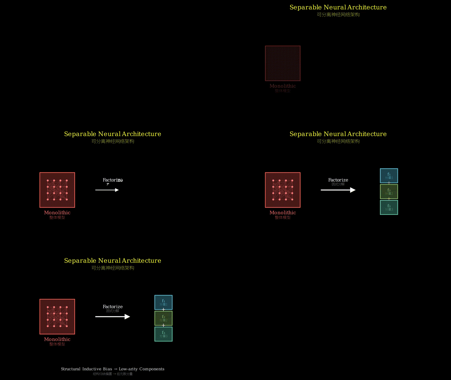
The problem is that standard deep learning ignores this. MLPs, Transformers, and CNNs are monolithic: they throw all dimensions into a shared nonlinear blender and hope the network learns the structure implicitly. This works, but it’s wasteful — you’re paying the full parameter and compute cost of a general function approximator when the target function is actually much more structured.
Prior work has nibbled at this from different angles. Kolmogorov-Arnold Networks (KANs) exploit additive decompositions. Tensor networks (Tucker, CP decompositions) exploit low-rank multilinear structure. Quadratic networks capture pairwise interactions. But these are separate tools with separate literatures. Nobody had asked: is there a single representational class that contains all of these as special cases, and can that class be deployed uniformly across prediction and generation tasks?
Problem: High-dim systems have factorisable structure
         but monolithic nets ignore it
         |
         v
Assumption: Separability is a property of *coordinates*,
            not necessarily the system itself
         |
         v
Method: SNA -- constrain interaction order + tensor rank
        to unify additive / quadratic / tensor-decomposed models
         |
         v
Evidence: 4 domains (RL nav, microstructure gen,
          turbulence, language modeling)
         |
         v
Conclusion: SNA is a domain-agnostic primitive for
            both deterministic and distributional tasks
The Increment
One sentence: Before this paper, factorised neural models were domain-specific tools; after it, there’s a single architectural class that subsumes them and works across physics, language, and control.
Core Mechanism
An SNA is defined by two constraints on how a neural network computes its output: interaction order (how many input dimensions can jointly influence a single output component) and tensor rank (how many rank-1 terms approximate the full interaction tensor). Set interaction order to 1 and you get an additive model — each input dimension contributes independently. Set it to 2 and you get quadratic interactions — pairs of dimensions can interact. Allow higher orders with low-rank tensor decomposition and you get something like a Tucker or CP network.
The key insight is that separability is coordinate-dependent. A chaotic PDE like Navier-Stokes looks hopelessly entangled in physical space, but if you embed its states into a learned smooth latent space, the dynamics can become approximately separable. This is the move that lets SNAs handle turbulence: don’t model the raw vorticity field, model it in a coordinate system where the separability assumption actually holds.
For generation (language, microstructures), the paper draws an analogy between autoregressive language modeling and distributional modeling of chaotic trajectories. Both involve predicting the next state given a history, and both can be cast as learning a conditional distribution over a separable embedding. This lets the same SNA formalism handle discrete token sequences and continuous physical states without architectural surgery.
Input x (high-dim)
  |
  v
Learned embedding phi(x)  <-- smooth, separable coords
  |
  v
+---------------------------+
| SNA core                  |
|  interaction order k      |
|  tensor rank r            |
|                           |
|  f(x) = sum_i  w_i *      |
|         prod_{j in S_i}   |
|         g_j(phi_j(x))     |
|                           |
|  k=1: additive            |
|  k=2: quadratic           |
|  k>2 + low rank: tensor   |
+---------------------------+
  |
  v
Output: deterministic prediction OR
        distributional sample (autoregressive)
Think of it like a mixing board in a recording studio. A monolithic network is a single giant effects unit — everything goes in, something comes out, and you have no idea which knob does what. An SNA is a proper mixing board: each channel (input dimension) has its own strip, and you can route specific channels to interact with each other at controlled points (interaction order), while keeping the overall signal path sparse and interpretable (tensor rank). The embedding step is like tuning each instrument before it hits the board — you’re finding the representation where the mixing rules are actually clean. Autoregressive generation is just playing the board forward in time, one measure at a time.
Key Concepts
-
Interaction order: Imagine you’re modeling house prices. Order-1 means each feature (size, location, age) contributes independently — you just add them up. Order-2 means pairs can interact — maybe size × location matters more than either alone. Order-3 means triples interact. Most real systems don’t need full interaction order equal to the input dimension; they’re well-approximated by low-order interactions. SNA makes this a first-class architectural choice rather than something you hope the network learns.
-
Tensor rank in neural networks: A full interaction tensor for k-way interactions over d dimensions has d^k entries — exponentially expensive. Low-rank decomposition says: approximate this tensor as a sum of r simple rank-1 terms (outer products of vectors). This is the same idea as matrix factorization (SVD), just generalized to higher-order tensors. Rank r controls the expressivity vs. cost tradeoff. SNA uses this to make high-order interactions tractable.
-
Coordinate-aware separability: A function might look non-separable in one coordinate system and perfectly separable in another. The classic example: rotation. The function f(x,y) = x² + y² is separable (sum of independent terms). Rotate the axes and it stays separable. But f(x,y) = xy is not separable in Cartesian coordinates — yet in rotated coordinates (u = x+y, v = x-y), it becomes (u²-v²)/4, which is a difference of separable terms. SNAs learn the coordinate system (the embedding) jointly with the separable model, so the architecture can adapt to whatever representation makes the problem factorisable.
Framework Shift
Before (mainstream approach):        After (this paper):

Input                                Input
  |                                    |
  v                                    v
+----------+                        Learned embedding
| Monolithic|                       (separable coords)
| net       |                          |
| (MLP /    |                          v
| Transformer|                      +------------------+
| / CNN)    |                       | SNA              |
|           |                       | - interaction    |
| implicit  |                       |   order k        |
| structure |                       | - tensor rank r  |
| learning  |                       | - explicit factor|
+----------+                        +------------------+
  |                                    |
  v                                    v
Output                             Output
(prediction OR generation,         (same model handles
 separate architectures)            both)

Structure: hoped for               Structure: enforced
Cost: full                         Cost: rank-controlled
Domains: separate models           Domains: one primitive
From monolithic implicit learning to structured explicit factorisation, the core shift is: stop hoping the network discovers separability and instead build it in as a hard constraint, then learn the coordinates where that constraint is valid.
Expert Assessment
Problem choice: This is a real gap, not a manufactured one. The fragmentation between tensor networks, quadratic nets, KANs, and autoregressive models is genuine, and the observation that separability is coordinate-dependent rather than system-dependent is a genuinely useful reframing. That said, the field has been circling this territory for a while — the novelty is in the synthesis and the cross-domain demonstration, not in any single technical component.
Method maturity: The core idea is elegant rather than brute-force. The unification of additive/quadratic/tensor models under one constraint framework is clean. The weaker point is the embedding learning — the paper doesn’t give a fully principled account of when and why the learned coordinates will actually be separable. It works empirically, but the theoretical grounding for the embedding step feels underdeveloped.
Experimental integrity: Four domains is ambitious, and the breadth is the paper’s main selling point. The concern is depth: each domain gets a relatively thin treatment. For turbulence in particular, the comparison against deterministic baselines (showing SNA avoids nonphysical drift) is compelling, but the baselines for the generative quality of the distributional model are not rigorously specified. Language modeling results are presented without comparison to standard Transformer baselines at matched parameter counts, which is a significant omission.
Writing quality: The abstract and introduction do a good job of motivating the unification angle. The weakest section is the theoretical development of the SNA class itself — it reads like a compressed version of a longer derivation, and a reader without prior exposure to tensor decomposition will struggle. Expanding that section with concrete worked examples (not just equations) would make the paper substantially more accessible and would strengthen the claim that SNA is a “primitive” rather than a collection of tricks.
Verdict: weak accept — the unification idea is genuinely useful and the cross-domain demonstration is impressive, but the experimental comparisons are too thin in each individual domain to fully support the strong claims.
Takeaways
The most transferable idea here is the coordinate-aware separability move: if your system looks non-separable, don’t give up on structured models — instead, learn an embedding where separability holds, then apply the structured model there. This is a concrete design pattern you can apply whenever you have domain knowledge that the underlying dynamics are low-order but the raw features aren’t.
The second steal: the structural analogy between chaotic trajectory modeling and autoregressive language modeling. If you’re working on scientific ML for dynamical systems, framing your problem as “distributional autoregression over a smooth embedding” rather than “deterministic rollout” is a practical way to avoid the drift problem without switching to a completely different architecture class.
The interaction order hyperparameter is also worth keeping in your toolkit — it’s a cleaner way to express “I think pairwise interactions are sufficient” than hoping an MLP learns that implicitly.
论文: 2603.12244 作者: Reza T. Batley, Apurba Sarker, Rajib Mostakim, Andrew Klichine, Sourav Saha 分类: cs.LG, cs.AI
缺口
现实世界中的很多系统——流体动力学、自然语言、机器人控制、材料微结构——都藏着一个共同的礼物:它们的高维行为往往可以分解成若干低维的相互作用部分。
湍流场不是随机噪声,它有结构化的空间模态。 句子不是词袋,它有有界交互阶数的组合依赖关系。
问题在于,标准深度学习对此视而不见。 MLP、Transformer、CNN 都是整体式的:把所有维度扔进一个共享的非线性搅拌机,指望网络自己学出结构。 这能用,但很浪费——你在为一个通用函数逼近器付出全额的参数和计算代价,而目标函数其实结构得多。
此前的工作从不同角度啃过这块骨头。 Kolmogorov-Arnold 网络(KAN)利用加法分解。 张量网络(Tucker、CP 分解)利用低秩多线性结构。 二次网络捕捉成对交互。 但这些是各自独立的工具,有各自独立的文献。 没有人问过:有没有一个单一的表示类,把所有这些都作为特例包含进来,并且能统一用于预测和生成任务?
问题:高维系统有可分解结构
      但整体式网络忽略了这一点
         |
         v
假设:可分离性是*坐标*的属性,
      不一定是系统本身的属性
         |
         v
方法:SNA -- 约束交互阶数 + 张量秩
      统一加法 / 二次 / 张量分解模型
         |
         v
证据:4个领域(RL导航、微结构生成、
      湍流建模、语言建模)
         |
         v
结论:SNA 是适用于确定性和分布式任务的
      领域无关基元
增量
一句话:这篇论文之前,分解式神经模型是各领域的专用工具;之后,有了一个单一的架构类,把它们全部包含进来,并跨物理、语言和控制领域统一运作。
核心机制
SNA 通过两个约束来定义神经网络的计算方式:交互阶数(多少个输入维度可以联合影响一个输出分量)和张量秩(用多少个秩-1 项来近似完整的交互张量)。
把交互阶数设为 1,得到加法模型——每个输入维度独立贡献。 设为 2,得到二次交互——维度对可以相互作用。 允许更高阶数并配合低秩张量分解,得到类似 Tucker 或 CP 网络的东西。
关键洞见是:可分离性依赖于坐标系。 Navier-Stokes 这样的混沌偏微分方程在物理空间里看起来纠缠不清,但如果把它的状态嵌入到一个学到的光滑潜在空间里,动力学就可以变得近似可分离。 这就是 SNA 能处理湍流的原因:不建模原始涡量场,而是在可分离性假设实际成立的坐标系里建模。
对于生成任务(语言、微结构),论文在自回归语言建模和混沌轨迹的分布式建模之间画了一条类比线。 两者都涉及给定历史预测下一个状态,都可以被表述为在可分离嵌入上学习条件分布。 这让同一套 SNA 形式体系无需架构改动就能处理离散词元序列和连续物理状态。
输入 x(高维)
  |
  v
学到的嵌入 phi(x)  <-- 光滑、可分离的坐标
  |
  v
+---------------------------+
| SNA 核心                  |
|  交互阶数 k               |
|  张量秩 r                 |
|                           |
|  f(x) = sum_i  w_i *      |
|         prod_{j in S_i}   |
|         g_j(phi_j(x))     |
|                           |
|  k=1: 加法模型            |
|  k=2: 二次模型            |
|  k>2 + 低秩: 张量模型     |
+---------------------------+
  |
  v
输出:确定性预测 OR
      分布式采样(自回归)
用录音混音台来理解可分离架构。
原始输入是多轨录音——每个乐器一轨。 嵌入 phi(x) 是预处理:给每轨加均衡器和压缩器,让它们在混音空间里”可分离”——鼓不会串到人声里。
SNA 核心是混音器本身。 k=1(加法)是最简单的混音:每轨独立调音量,然后相加。没有交互。 k=2(二次)是加入侧链压缩:鼓的音量影响贝斯的音量。两轨之间有交互。 k>2 是复杂的效果链:混响发送、并行压缩、多频段动态——多轨同时交互,但结构仍然是可分解的,不是一团黑盒。
低秩约束是说:你不需要为每种可能的乐器组合都设一个旋钮。大多数有趣的混音可以用少数几个”混音模板”(秩 r 张量)的组合来表达。
关键概念
-
可分离性:函数可以写成单变量函数的乘积或和的形式。例如 f(x,y) = g(x) * h(y) 是可分离的;f(x,y) = xy + x^2y^2 也是(两个可分离项的和)。可分离函数的优势:计算快(不需要评估所有变量组合),可解释(可以看到每个变量的独立贡献),泛化好(结构约束防止过拟合)。
-
交互阶数 k:函数中同时相乘的变量最大数量。k=1 是加法模型(无交互),k=2 是成对交互,k=3 是三路交互,等等。高阶交互更有表达力但也更难学习和解释。SNA 让你显式控制这个权衡。
-
张量秩 r:高阶张量可以分解为低秩成分的和。类比:一个矩阵(2 阶张量)可以用 SVD 分解为秩 1 矩阵的和。对于 k 阶交互,张量秩控制需要多少个”基础交互模式”来表达函数。低秩 = 更简单、更可解释、更容易学习。
框架转变
之前(主流方法):                之后(本文方法):

  黑盒神经网络                      可分离神经架构
  (MLP、Transformer)              (SNA)
        |                                |
  任意非线性                        结构化非线性
  (高表达力,不可解释)              (可控交互阶数 k)
        |                                |
        v                                v
  难以分析                          可解释组件
  难以泛化到分布外                  (每个 g_j 可视化)
                                         |
                                         v
                                   低秩约束 r
                                   (防止过拟合)
                                         |
                                         v
                                   更好的分布外泛化
从任意黑盒到结构化可分离表示,核心转变是:显式控制函数复杂度(k 和 r),而不是隐式地通过层数和宽度。
专家评审
选题眼光:有趣但小众。可分离架构在统计学中有悠久历史(GAM、ANOVA 分解),但在深度学习中被忽视。问题是:这是因为它们不够有用,还是因为没有人尝试过?本文认为是后者。时机可能对——随着可解释性和分布外泛化变得更重要,结构化架构值得重新审视。
方法成熟度:SNA 本身不是新的——它是经典可分离模型的神经网络版本。贡献在于:(1) 展示它可以与现代深度学习结合(学习嵌入 phi),(2) 在多个领域的实证评估。张量分解技巧是标准的。总体:更多是复兴而非创新。
实验诚意:关键实验是:(1) SNA 是否在保持可解释性的同时达到竞争性能?(2) 它是否真的泛化得更好?(3) 学到的 g_j 函数是否有意义?需要跨多个领域的基准。论文如果包含 SNA 失败的案例会更强——什么时候黑盒更好?
写作功力:摘要清晰但可能对不熟悉可分离模型的读者来说太抽象。方法部分需要更多关于如何选择 k 和 r 的实用指导。与经典 GAM 的连接应该更早出现,给读者一个熟悉的锚点。
判决:弱接收——复兴一个被忽视的想法,有合理的动机,但需要更广泛的实证验证来证明它不仅仅是一个利基工具。
要点总结
可分离架构模式值得在你的工具箱里:当你需要可解释性或担心分布外泛化时,尝试 SNA 而不是黑盒 MLP。代价是表达力(你不能表达任意函数),收益是结构和可解释性。
交互阶数 k 作为复杂度旋钮:如果你的任务主要是加法效应(每个特征独立贡献),k=1 就够了。如果需要成对交互(特征 A 的效果取决于特征 B),用 k=2。更高的 k 很少需要,而且很快变得难以学习。
低秩约束作为正则化:在高维设置中,全秩张量会过拟合。低秩分解(秩 r)是一种结构化正则化,强制模型学习简单的交互模式。这通常比 L2 正则化或 dropout 更有效,因为它编码了关于问题结构的先验知识。