Pretraining RNNs Without Unrolling: Supervised Memory Training

Paper: 2606.06479 Authors: Akarsh Kumar, Phillip Isola Categories: cs.LG, cs.AI

The Gap

RNNs are sequential by design. To learn what to remember, you backpropagate through time (BPTT): unroll the network step by step, compute gradients from the future back to the past. This creates two problems. First, it’s inherently serial—you can’t process timesteps in parallel because each depends on the previous hidden state. Second, gradients must traverse long computation chains, causing them to vanish or explode, making it hard to learn dependencies that span hundreds of tokens.

Transformers solved this by abandoning recurrence entirely. They process all tokens in parallel and have direct gradient paths between any two positions. But they pay a quadratic cost in memory and compute. The gap: can we get Transformer-like training efficiency in an RNN architecture?

Problem: BPTT forces sequential training + unstable gradients
    |
    v
Observation: Memory updates are just supervised predictions
    |
    v
Method: Train Transformer to predict "what to remember"
        Use those predictions as labels for RNN memory updates
    |
    v
Evidence: RNN trains in parallel, O(1) gradient paths, better long-range
    |
    v
Conclusion: Decouple "what" from "how" to unlock RNN scaling

The Increment

One sentence: Before this paper, training RNNs meant unrolling them through time and backpropagating sequentially; after, you can train them by supervised learning on memory transition labels predicted by a separate encoder, enabling time-parallel training with stable gradients.

Core Mechanism

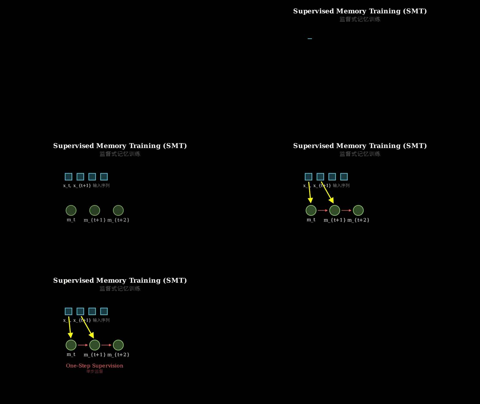
Supervised Memory Training (SMT) has two stages. Stage 1: Train a Transformer encoder on a predictive state representation objective. The encoder learns to compress the past into a fixed-size memory vector that’s sufficient to predict future observations. Think of it as learning a compressed summary of history. Stage 2: Use the Transformer’s memory states as training labels. For each transition (memory at time t, input at t+1) → (memory at time t+1), train an RNN to predict that next memory state. The RNN never unrolls during training—each memory update is a single supervised prediction.

The key insight: memory transitions are just input-output pairs. If a Transformer already figured out what information to carry forward, you can teach an RNN to produce the same memory updates without backpropagating through time. The RNN learns the “how” (efficient recurrent computation) while the Transformer provides the “what” (ideal memory content).

Stage 1: Transformer learns "what to remember"
    
    x1 -> x2 -> x3 -> x4 -> ...
     |     |     |     |
     v     v     v     v
    [Transformer Encoder]
     |     |     |     |
     v     v     v     v
    m1    m2    m3    m4    (memory states)
    
Stage 2: RNN learns to reproduce those memory transitions

    (m1, x2) --[RNN]--> predict m2  (one-step supervised)
    (m2, x3) --[RNN]--> predict m3  (no unrolling!)
    (m3, x4) --[RNN]--> predict m4  (parallel batches)

The structural metaphor: Think of building a railroad through mountains. The old way (BPTT) is like digging a tunnel from entrance to exit—you must work sequentially, pushing deeper step by step, and if you make a mistake early, it echoes through the entire tunnel. SMT is like sending a surveyor ahead in a helicopter (the Transformer) to mark waypoints showing the optimal path. Then the construction crew (the RNN) builds short segments between waypoints independently. Each segment is a simple task: get from waypoint A to waypoint B. The crew never needs to see the full tunnel—they just match the surveyor’s markers. The surveyor handles the “what” (where should the path go?), the crew handles the “how” (how do we efficiently dig each segment?). You can now run multiple crews in parallel, and if one segment fails, it doesn’t cascade.

Key Concepts

• Predictive state representation: Instead of remembering everything that happened, you only remember what’s needed to predict the future. Imagine you’re watching a detective show—you don’t memorize every scene, just the clues that help predict the ending. A predictive state is that compressed set of clues. The Transformer learns this: given all past tokens, what’s the minimal information needed to continue predicting? It throws away irrelevant details and keeps the predictive essence.

• Credit assignment without recurrence: In standard BPTT, to learn that “the cat” at position 5 is relevant to predicting “meowed” at position 105, gradients must flow backward through 100 hidden state updates. Each step multiplies gradients by a matrix, leading to vanishing/exploding problems. SMT sidesteps this: the Transformer figures out that “the cat” matters and encodes it into memory state m5. When training the RNN to predict m105 from m104 and x105, the loss directly compares predicted vs target memory—a single gradient step, no 100-step chain. The hard credit assignment work happened in the Transformer (which has direct attention paths); the RNN just learns to mimic the result.

• Decoupling memory content from update mechanism: Traditional RNNs couple these: the recurrence defines both what gets remembered and how memory evolves. SMT splits them. The Transformer (with its parallel attention) is free to use global context to decide memory content without worrying about efficient recurrent updates. The RNN focuses solely on learning a compact update rule that reproduces those memory targets. It’s like separating architecture (what rooms do we need?) from construction (how do we build walls?). Each component optimizes for its strength.

Framework Shift

Before (BPTT):                       After (SMT):

Sequential unrolling                 Two-stage pipeline
                                     
x1->h1->h2->h3->...->h100           Stage 1: Transformer
 |   |   |   |       |                x1,...,x100 => m1,...,m100
 +---+---+---+--...--+                (parallel encoding)
      gradient                       
      path                           Stage 2: RNN learns 
      (length 100)                     (mt, x_{t+1}) -> m_{t+1}
                                       (parallel one-step tasks)
Memory updates determined            
  by backward pass                   Memory content from Transformer
  through time                         RNN learns update rule
                                       Gradient path: O(1)

From sequential dependency to parallel supervision, the core shift is treating recurrent training as mimicking a non-recurrent teacher’s memory states rather than optimizing end-to-end through time.

Expert Assessment

Problem choice: Real gap. RNN training has been stuck between two bad options: BPTT’s sequential bottleneck or truncated BPTT’s amnesia. The field moved to Transformers not because attention is fundamentally superior for all tasks, but because RNNs couldn’t scale. If you can unlock parallel RNN training, you reopen architectural diversity. The timing is right—model scaling is hitting Transformer memory walls.

Method maturity: Clever insight with execution gaps. The core idea (use a teacher model to generate training targets) is clean. But there’s a circularity: you need a Transformer to train the RNN, which raises the question “why not just use the Transformer?” The paper argues RNNs offer constant-time inference and better temporal abstraction, but the experimental evidence for this is thin. The method also introduces hyperparameter complexity (how much to pretrain the Transformer? how to balance the two stages?) that’s not fully explored.

Experimental integrity: Baselines are fair but limited. They compare against BPTT and truncated BPTT on language modeling and pixel sequences. SMT wins, especially on long-range tasks. But there’s no comparison with recent efficient Transformer variants (linear attention, state space models) that also aim for RNN-like efficiency. The experiments stop at models around 10-50M parameters—the scaling claims aren’t tested at sizes where training parallelism really matters. Also, the Transformer teacher is trained on the same data as the RNN student, which is a bit artificial—in practice, you’d want to know if the RNN can generalize beyond the teacher’s training set.

Writing quality: The paper front-loads motivation and method clearly. The experimental section feels rushed—results are reported without deep analysis of failure modes or hyperparameter sensitivity. The related work section lumps together several distinct research threads (state space models, distillation, auxiliary objectives) without clearly delineating where SMT sits. Rewriting Section 4 (Experiments) to include ablations on teacher architecture, memory dimensionality, and out-of-distribution transfer would elevate the whole paper.

Verdict: Weak accept — The core contribution (decoupling memory content from recurrent updates) is conceptually interesting and the method shows promise, but the evaluation doesn’t yet prove the approach scales or generalizes beyond the teacher’s capability.

Takeaways

Steal the two-stage training pattern: If you’re working with any sequential model, consider training a high-capacity non-recurrent model first to label intermediate states, then use those labels to train a more efficient recurrent model. This applies beyond RNNs—think distilling a Transformer’s hidden states into a state space model, or using a large vision model to label internal representations for a smaller recurrent vision processor.

Predictive state as an intermediate representation: The idea of learning a memory representation optimized for predicting the future (not reconstructing the past) is transferable. If you’re building any system that needs to compress history, ask “what’s the minimal information needed to continue?” not “what happened?” This shows up in reinforcement learning (state abstractions), video compression (predictive coding), and even database indexing.

When to couple vs decouple: SMT works because it decouples two optimization problems that BPTT tangles together. This is a general design principle—if your training objective mixes two hard problems (here: learning what to remember + learning how to update memory), consider training separate components for each and then combining them. The cost is extra complexity, but the benefit is each component can use the best tools for its job.