Posterior Augmented Flow Matching: Training Generative Models with Multiple Target Trajectories

Paper: 2605.00825 Authors: George Stoica, Sayak Paul, Matthew Wallingford, Vivek Ramanujan, Abhay Nori, Winson Han, Ali Farhadi, Ranjay Krishna, Judy Hoffman Categories: cs.CV

The Gap

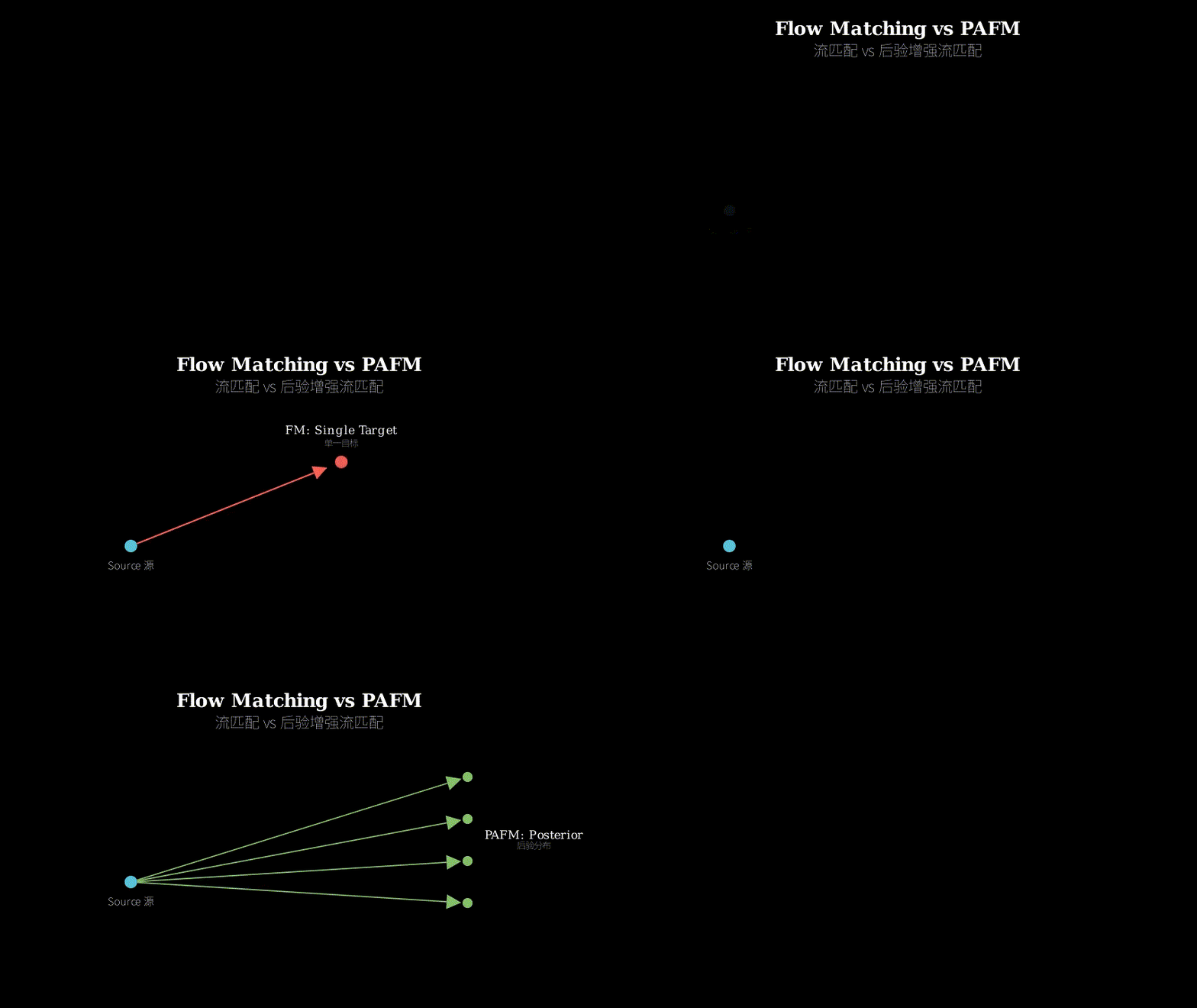
Flow matching (FM) trains generative models by learning a vector field that transports noise to data. The method is elegant: pair each noise sample with a data sample, interpolate between them, and train a network to predict the velocity at each point along the path. But there’s a problem hiding in plain sight.

In high-dimensional spaces like 512×512 images, each training sample supervises exactly one trajectory through an astronomically large state space. You’re learning a vector field over billions of dimensions from single-point observations scattered sparsely across it. The result: flow collapse. The model memorizes specific source-target pairings instead of learning the underlying distribution structure. Different noise samples that should map to diverse outputs collapse to nearly identical results.

Prior work tried to fix this with better coupling strategies (optimal transport, minibatch coupling) or architectural improvements. But they all share the same fundamental constraint: one training sample = one supervision signal = one trajectory.

Problem: Sparse supervision in high-D space
   |
   v
Assumption: Each intermediate state has multiple valid completions
   |
   v
Method: Supervise with expectation over posterior of valid targets
   |
   v
Evidence: 3.4 FID improvement across architectures/scales
   |
   v
Conclusion: Multi-target supervision reduces variance, prevents collapse

The Increment

One sentence: Before PAFM, each training sample taught the model one path through latent space; after PAFM, each sample teaches an ensemble of plausible paths weighted by their likelihood.

Core Mechanism

Standard FM works like this: given a noise sample x₀ and data sample x₁, interpolate to get xₜ at time t, then train a network to predict the velocity vₜ that points from xₜ toward x₁. The loss is simple: match the predicted velocity to the ground truth direction.

PAFM keeps this structure but replaces the single target x₁ with a weighted mixture of multiple candidate targets. For each intermediate state xₜ and condition c (like a class label or text prompt), PAFM constructs an approximate posterior over which endpoints x₁ could plausibly have led to xₜ.

The posterior factorizes into two terms: (1) the likelihood p(xₜ | x₁, c) — how probable is this intermediate given that endpoint? — and (2) the prior p(x₁ | c) — how probable is that endpoint given the condition? PAFM uses a pre-trained diffusion model to evaluate both terms. For likelihood, it runs the diffusion model’s denoising process starting from xₜ and measures how well it reconstructs x₁. For the prior, it samples from the diffusion model conditioned on c.

The training objective becomes an expectation over this posterior. In practice, PAFM uses importance sampling: sample K candidate endpoints from the prior, weight them by their likelihoods, and train the flow model to match a mixture of velocities pointing toward all K targets. The weights ensure that more plausible completions contribute more to the gradient.

Training step:

  x0 (noise) ----[interpolate]----> xt (intermediate)
                                     |
                                     v
                            [sample K candidates]
                                     |
                    +----------------+----------------+
                    |                |                |
                   x1_1             x1_2    ...     x1_K
                    |                |                |
              [weight by p(xt|x1_1)] ...   [weight by p(xt|x1_K)]
                    |                |                |
                    +-------[mixture]--------+
                                     |
                                     v
                            [aggregate velocity]
                                     |
                                     v
                            [train flow model]

Think of it like learning to navigate a city. Standard FM is like having one person tell you “from this intersection, go toward the library.” But what if multiple destinations are equally valid from that intersection? PAFM is like asking several locals where they’re headed, weighting their advice by how confident they seem, and learning the average direction. The library-goer’s advice counts more if the intersection is clearly on the way to the library. The museum-goer’s advice counts less if you’d have to backtrack. By aggregating multiple plausible routes, you learn the underlying street network instead of memorizing one person’s commute.

Key Concepts

• Flow collapse: When a generative model maps diverse inputs to overly similar outputs, failing to capture the full diversity of the target distribution. In flow matching, this happens because each training sample supervises only one trajectory through latent space. The model learns to reproduce specific source-target pairings it saw during training rather than the general structure of how noise transforms into data. Imagine training a model to draw faces by showing it exactly one path from random scribbles to each face in your dataset. The model might learn “when you see this scribble pattern, draw this specific face” instead of “when you see nose-like features emerging, refine them into a realistic nose.” The result: different starting scribbles collapse to the same few faces the model memorized.

• Posterior over valid completions: Given an intermediate state xₜ and a condition c, there are many possible endpoints x₁ that could have produced xₜ through the forward interpolation process. The posterior p(x₁ | xₜ, c) captures this uncertainty. PAFM approximates this posterior by factorizing it: p(x₁ | xₜ, c) ∝ p(xₜ | x₁, c) × p(x₁ | c). The likelihood term p(xₜ | x₁, c) asks “if we were heading toward x₁, how likely would we be at xₜ right now?” The prior term p(x₁ | c) asks “how likely is x₁ as an endpoint given the condition?” Concretely, if you’re generating an image of a dog and you’re halfway through the process, the posterior captures all the different dog images you could plausibly be heading toward, weighted by how well each one explains your current intermediate state.

• Importance sampling for gradient aggregation: Computing the exact expectation over the posterior is intractable because there are infinitely many possible endpoints. PAFM uses importance sampling: sample K candidates from an easy-to-sample proposal distribution (the prior p(x₁ | c)), then reweight each candidate by the likelihood ratio. This gives an unbiased estimate of the expectation while keeping computation tractable. The key insight: you don’t need to sample from the true posterior directly. Sample from something close (the prior), then correct for the mismatch with weights. In practice, this means generating K plausible endpoints using a pre-trained diffusion model, evaluating how well each explains the intermediate state, and training the flow model to match a weighted average of velocities toward all K targets.

Framework Shift

Before (standard FM):                After (PAFM):

x0 -----> xt -----> x1               x0 -----> xt -----> x1_1 (w1)
  (noise)  |      (data)               (noise)  |      \ x1_2 (w2)
           |                                    |       \ x1_3 (w3)
           v                                    |        ...
      [predict v_t]                             |       \ x1_K (wK)
           |                                    |
      [loss: ||v_t - (x1-xt)||]                v
                                           [predict v_t]
Single trajectory supervision                  |
High variance, memorization              [loss: ||v_t - Σ w_i(x1_i-xt)||]

                                         Multi-trajectory supervision
                                         Lower variance, generalization

From single-target supervision to posterior-weighted ensemble, the core shift is replacing point estimates with distributions over plausible completions.

Expert Assessment

Problem choice: This is a real gap. Flow collapse is a known failure mode in flow-based generative models, and the paper correctly identifies the root cause: under-constrained supervision in high-dimensional spaces. The problem sits at the intersection of two active research threads — improving flow matching efficiency and addressing mode collapse in generative models. Not groundbreaking problem formulation, but solid and timely.

Method maturity: The core idea is elegant: if one target gives a noisy gradient, average over multiple targets to reduce variance. The theoretical grounding (unbiased estimator, variance reduction proof) is clean. However, the method introduces a dependency on a pre-trained diffusion model for posterior evaluation, which feels like trading one problem for another. Why not train the flow model to be its own posterior evaluator? The importance sampling scheme is standard, not novel. The real contribution is recognizing that multi-target supervision is tractable and beneficial.

Experimental integrity: Baselines are fair — they compare against standard FM with the same architectures and training budgets. The improvements (up to 3.4 FID) are consistent across different scales (SiT-B/2, SiT-XL/2) and architectures (SiT, MMDiT), which strengthens the claim. The ablations (varying K, different weighting schemes) are thorough. One red flag: the method requires a pre-trained diffusion model, but the paper doesn’t deeply analyze how the quality of that model affects PAFM’s performance. If the diffusion model is weak, does PAFM degrade gracefully or collapse?

Writing quality: The paper is well-structured and the motivation is clear. The theoretical section (Section 3) is dense but rigorous. However, Section 4 (method details) buries important implementation choices in paragraphs when a clear algorithm box would help. The related work section is thorough but could be trimmed — some citations feel like box-checking rather than building narrative. If I were rewriting, I’d expand Section 5.3 (ablations) with more analysis of failure cases and the diffusion model dependency.

Verdict: weak accept — Solid incremental contribution with consistent empirical gains, but the reliance on pre-trained diffusion models limits the method’s independence and the novelty is more in application than in algorithmic innovation.

Takeaways

Multi-target supervision as variance reduction: The core trick — replacing single-sample supervision with a weighted ensemble of plausible targets — transfers beyond flow matching. Anytime you’re training a model with sparse, high-variance supervision signals (e.g., reinforcement learning, one-shot imitation learning), consider whether you can construct a distribution over plausible targets and train against the expectation. The key is having a way to evaluate the likelihood of each candidate target.

Factorizing intractable posteriors: PAFM’s posterior factorization (likelihood × prior) is a textbook move, but the paper shows it’s practical even when both terms require expensive model evaluations. If you have a generative model that can sample from p(x|c) and evaluate p(y|x,c), you can approximate p(x|y,c) via importance sampling without training a separate inverse model. This pattern shows up in inverse problems, Bayesian inference, and guided generation.

Pre-trained models as auxiliary supervisors: Using a diffusion model to provide richer supervision for a flow model is a specific instance of a broader strategy: leverage a strong pre-trained model not as the final solution, but as a teacher or evaluator during training. The diffusion model here acts like an oracle that says “here are plausible completions and how likely they are.” This is cheaper than distillation (no need to match the teacher’s full behavior) and more flexible than fixed augmentation (the supervision adapts to each training sample).