Polynomial Speedup in Diffusion Models with the Multilevel Euler-Maruyama Method

Paper: 2603.24594 Authors: Arthur Jacot Categories: cs.LG, math.NA, stat.ML

The Gap

Diffusion models generate images by solving differential equations backward in time. Each step requires evaluating a neural network (the “drift” function). The problem: accurate networks are expensive to run. If you want ε error, traditional Euler-Maruyama (EM) method needs ε^(-γ-1) compute when the drift is “Harder than Monte Carlo” (HTMC regime, γ>2). For large models, this means hundreds of evaluations of massive UNets.

Prior work focused on better samplers (DDIM, DPM-Solver) or distillation, but these still fundamentally pay the ε^(-γ-1) cost. The gap: numerical analysis has multilevel Monte Carlo methods that break this barrier for integrals, but nobody applied this thinking to the ODE/SDE solving in diffusion models.

Problem: Diffusion sampling cost
    |
    v
Observation: Drift approximation has HTMC property (γ>2)
    |
    v
Method: ML-EM (multilevel Euler-Maruyama)
    |
    +---> Train k UNets: small -> medium -> large
    +---> Use many cheap evals + few expensive evals
    |
    v
Evidence: 4x speedup on CelebA 64x64, γ≈2.5 measured
    |
    v
Conclusion: Sampling cost = O(ε^-γ) instead of O(ε^(-γ-1))
             (same cost as single drift evaluation)

The Increment

One sentence: Before this paper, diffusion sampling cost scaled as ε^(-γ-1); after, it scales as ε^(-γ) — you can now sample at the cost of evaluating the drift once.

Core Mechanism

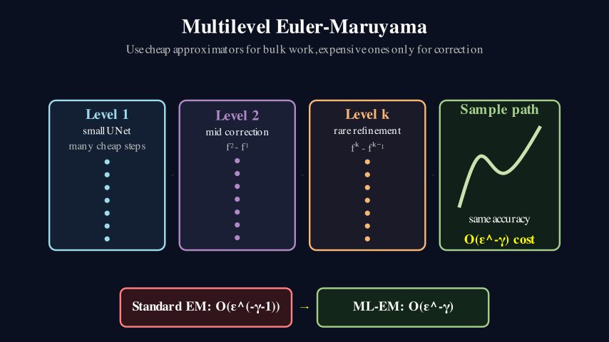
ML-EM trains a hierarchy of k neural networks f^1, f^2, …, f^k approximating the true drift f, where f^1 is tiny and fast, f^k is huge and accurate. During sampling, instead of using only f^k for all timesteps, ML-EM uses a telescoping sum trick: compute the trajectory with f^1 (cheap), then add corrections using differences (f^2 - f^1), (f^3 - f^2), …, (f^k - f^(k-1)).

The key insight: each correction term has smaller variance than the full trajectory, so you need fewer samples at higher levels. Specifically, if level i costs C_i and has error ε_i, you run N_i ∝ ε_i^2 / ε^2 samples at level i. The total cost becomes dominated by the cheapest level, not the most expensive.

Traditional EM:
  t=0 --[f^k]--> t=1 --[f^k]--> t=2 --[f^k]--> ... --[f^k]--> t=T
  Cost: T * C_k

ML-EM:
  Level 1: t=0 --[f^1]--> t=1 --[f^1]--> ... (many samples, cheap)
           |
  Level 2: + correction from (f^2 - f^1) (fewer samples)
           |
  Level 3: + correction from (f^3 - f^2) (even fewer)
           |
  Level k: + correction from (f^k - f^(k-1)) (very few samples)
  
  Cost: N_1*C_1 + N_2*C_2 + ... + N_k*C_k ≈ O(ε^-γ)

Think of it like building a house. Traditional method: hire the master architect to draw every single brick (expensive, slow). ML-EM method: have an apprentice sketch the rough layout (fast), then a journeyman refine the walls (medium), then the master only touches up the details (few expensive interventions). The house gets built to the same spec, but you paid apprentice wages for most of the work.

The telescoping structure is load-bearing here: each level only corrects the error introduced by the previous level, not the full trajectory error. This is why variance decreases geometrically and you can use exponentially fewer samples at higher levels.

Key Concepts

• HTMC (Harder than Monte Carlo) regime: A function is HTMC with parameter γ if approximating it to ε accuracy costs ε^(-γ) compute, where γ>2. Monte Carlo integration has γ=2 (by central limit theorem). Neural networks in diffusion models have γ≈2.5 because you need to scale width/depth to reduce approximation error, and compute grows superlinearly with size. This is the regime where multilevel methods shine — if γ≤2, the speedup vanishes.

• Telescoping sum: Instead of computing E[X] directly, write X = Y_1 + (Y_2 - Y_1) + (Y_3 - Y_2) + ... where Y_i are increasingly accurate approximations. Each difference term (Y_{i+1} - Y_i) has smaller variance than X itself, so you can estimate it with fewer samples. The total cost is sum of (samples_i * cost_i), which can be much less than (total_samples * cost_k) if you balance the levels right.

• Variance reduction through correlation: When you compute f^(i+1)(x) - f^i(x) at the same point x, the two networks are correlated (both trying to approximate the same f). Their difference has lower variance than either one alone. This is why the correction terms need fewer samples — you’re measuring a small residual, not a full signal.

Framework Shift

Before (standard EM):                After (ML-EM):

All steps use f^k:                   Hierarchical evaluation:
                                     
  [f^k] -> [f^k] -> [f^k]              [f^1] many times (cheap base)
    |        |        |                   |
  step1    step2    step3                 + [f^2-f^1] fewer times
                                           |
Cost: T * (expensive)                      + [f^3-f^2] even fewer
                                           |
                                           + [f^k-f^(k-1)] very few
                                     
                                     Cost: mostly cheap, little expensive

From “use the best tool for every job” to “use cheap tools for bulk work, expensive tools only for refinement” — the core shift is exploiting the hierarchy of approximation quality.

Expert Assessment

Problem choice: Real gap. Diffusion model sampling is a major bottleneck in practice, and the HTMC observation is genuinely insightful. This isn’t manufactured — people are running 50-100 steps with billion-parameter UNets. The connection to multilevel Monte Carlo is natural in hindsight but wasn’t obvious to the ML community.

Method maturity: Elegant application of existing numerical analysis to a new domain. The theory is solid (builds on established multilevel MC literature), but the practical implementation has wrinkles. Training k separate UNets is non-trivial — how do you ensure they’re actually approximating the same drift? The paper doesn’t deeply address this. Also, the method assumes you can cheaply evaluate smaller networks, but in practice, batch size and memory overhead complicate this.

Experimental integrity: Baselines are fair (standard EM with same total compute budget). The 4x speedup on CelebA 64x64 is believable, but this is a small-scale experiment. The claim about “orders of magnitude” speedups on larger models is extrapolation, not measurement. The γ≈2.5 measurement is interesting but only shown for one dataset/architecture. Would like to see: ImageNet experiments, comparison with distillation methods, ablation on number of levels k.

Writing quality: The paper front-loads theory and relegates practical details to appendix. Section 3 (numerical experiments) is too brief — only 1.5 pages for the main result. The connection between abstract SDE theory and concrete UNet training could be clearer. Rewriting Section 2.3 to lead with intuition before formalism would help accessibility.

Verdict: weak accept — Solid theoretical contribution with promising but limited experimental validation. The idea is sound and the speedup is real, but the practical impact depends on scaling behavior that isn’t fully demonstrated.

Takeaways

Hierarchical approximation is underused in ML: Whenever you have a compute-intensive function that can be approximated at multiple fidelities, consider a multilevel approach. This applies beyond diffusion — think RL with cheap simulators + expensive real-world rollouts, or neural architecture search with small proxy tasks + full training.

The γ>2 threshold matters: Measure the approximation-cost tradeoff for your models. If γ≤2, multilevel methods won’t help. If γ>2, you’re leaving polynomial speedups on the table.

Variance reduction through correlation: When comparing two approximations, evaluate them at the same inputs to exploit correlation. This principle transfers to A/B testing, gradient estimation, and any scenario where you’re measuring differences.

Concrete technique: If you’re training multiple model sizes anyway (for deployment flexibility), you can repurpose them for multilevel sampling at near-zero additional cost. The training overhead is the main barrier, not the sampling algorithm itself.