PiD: Rethinking Latent Decoding as Pixel Diffusion for Fast High-Resolution Generation

Paper: 2605.23902 Authors: Yifan Lu, Qi Wu, Jay Zhangjie Wu, Zian Wang, Huan Ling, Sanja Fidler, Xuanchi Ren Categories: cs.CV

The Gap

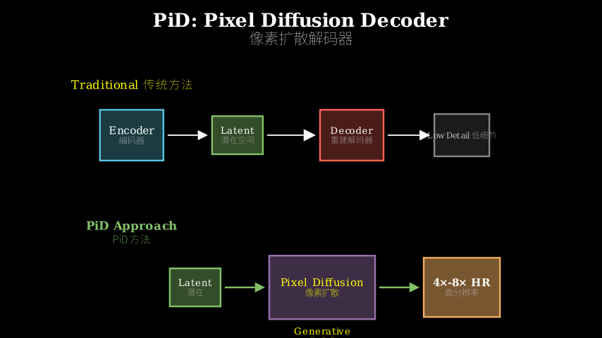
Current high-resolution text-to-image systems (Stable Diffusion, autoregressive models) generate in compact latent space, then decode latents to pixels using a VAE decoder. The decoder is trained for reconstruction—to invert the encoder—not to synthesize new details. At megapixel scale, this becomes a bottleneck: the decoder is expensive, and upsampling requires separate cascaded super-resolution models that add latency and memory overhead.

The gap: latent decoding and upsampling are treated as separate reconstruction tasks, not as opportunities for generative synthesis.

Problem: VAE decoder optimized for reconstruction, not detail synthesis
   |
   v
Assumption: Pixel diffusion can condition on latents and generate details
   |
   v
Method: PiD - pixel diffusion decoder with sigma-aware adapter
   |
   v
Evidence: 4-8× upscaling in <1s, 6× faster than cascaded SR, better quality
   |
   v
Conclusion: Unifying decoding + upsampling as conditional generation wins

The Increment

One sentence: Before PiD, latent decoding was reconstruction (VAE inverts encoder); after PiD, latent decoding is conditional generation (pixel diffusion synthesizes details while upscaling).

Core Mechanism

PiD has three components: (1) a pixel diffusion backbone that denoises directly in high-resolution pixel space, (2) a sigma-aware adapter that injects noise-corrupted latents as conditioning, and (3) optional DMD2 distillation to reduce inference to 4 steps.

The data flow: latent diffusion generates a low-resolution latent (e.g., 64×64 for a 512×512 image). Instead of passing this to a VAE decoder, PiD treats it as conditioning for pixel diffusion. The adapter adds noise to the latent (matching the current diffusion timestep’s noise level), then injects it into the pixel diffusion backbone via cross-attention or concatenation. The backbone denoises random noise at high resolution (2048×2048) conditioned on the noisy latent, synthesizing fine details that were never in the latent space.

Key operation: the adapter is “sigma-aware”—it corrupts the latent with noise proportional to the current diffusion timestep. This lets PiD decode partially denoised latents, so latent diffusion can terminate early (fewer steps) and hand off to PiD for the final detail synthesis.

Latent Diffusion (64x64)  -->  Noisy Latent
                                     |
                                     v
                            Sigma-Aware Adapter
                                     |
                                     v
Random Noise (2048x2048) --> Pixel Diffusion Backbone --> Clean Pixels
                                     ^
                                     |
                              (conditioned on latent)

Think of PiD like a sketch-to-painting process. The latent diffusion gives you a rough sketch (low-resolution latent). A traditional VAE decoder is like tracing over the sketch with a pen—it reproduces what’s there but adds no new information. PiD is like a painter who takes the sketch and paints a full canvas: the sketch guides composition and structure, but the painter adds brushstrokes, textures, and details that weren’t in the sketch. The sigma-aware adapter is like showing the painter a progressively clearer sketch—early on, the sketch is blurry (high noise), so the painter has more freedom; later, the sketch is sharper (low noise), so the painter follows it more closely.

Key Concepts

• Sigma-aware conditioning: In diffusion models, sigma (σ) represents the noise level at each timestep. Early in denoising, σ is high (lots of noise); late in denoising, σ is low (almost clean). PiD’s adapter adds noise to the latent proportional to the current σ. Why? If the pixel diffusion is at a noisy timestep but receives a clean latent, there’s a mismatch—the model doesn’t know how much to trust the latent. By corrupting the latent to match the current noise level, the adapter aligns the conditioning with the denoising process. Concrete example: at timestep t=800 (high noise), the latent is heavily corrupted, so the pixel diffusion uses it as a loose guide. At t=100 (low noise), the latent is nearly clean, so the pixel diffusion follows it closely. This enables early termination of latent diffusion—you can stop at t=400 in latent space and let PiD finish the job in pixel space.

• Latent vs pixel diffusion: Latent diffusion (Stable Diffusion) denoises in a compressed latent space (e.g., 64×64 for a 512×512 image), then decodes to pixels. Pixel diffusion denoises directly in pixel space (512×512 or higher). Why does this matter? Latent diffusion is fast because the space is small, but the VAE decoder is a fixed bottleneck—it can’t add details beyond what the encoder captured. Pixel diffusion is slower because the space is large, but it can synthesize arbitrary details. PiD combines both: use latent diffusion for coarse structure (fast), then pixel diffusion for fine details (expressive). The tradeoff: pixel diffusion at 2048×2048 is expensive, but PiD distills it to 4 steps, making it practical.

• DMD2 distillation: Diffusion models typically need 20-50 denoising steps. Distillation trains a student model to match the teacher’s output in fewer steps. DMD2 (Distribution Matching Distillation) is a recent technique that distills diffusion models to 4 steps by matching the distribution of generated samples, not just individual outputs. PiD applies DMD2 to the pixel diffusion backbone, reducing inference from ~20 steps to 4 steps. This is critical for real-time use—without distillation, pixel diffusion at 2048×2048 would be too slow. With distillation, PiD decodes in under 1 second on consumer hardware.

Framework Shift

Before (VAE decoder):                After (PiD):

Latent Diffusion                     Latent Diffusion
       |                                    |
       v                                    v
  VAE Decoder                         Sigma-Aware Adapter
       |                                    |
       v                                    v
  Pixels (512x512)                   Pixel Diffusion (2048x2048)
       |                                    |
       v                                    v
Cascaded SR Model                    Pixels (2048x2048)
       |
       v
  Pixels (2048x2048)

(reconstruction → upsampling)        (conditional generation)

From two-stage reconstruction (decode then upscale) to single-stage conditional generation (decode and upscale simultaneously), the core shift is treating the decoder as a generative model, not an inverse function.

Expert Assessment

Problem choice: Real gap. VAE decoders are indeed reconstruction-oriented and become a bottleneck at megapixel scale. Cascaded super-resolution adds latency and memory. The field has been moving toward pixel diffusion (e.g., Imagen, PixArt), but those are full pixel-space models—PiD’s insight is to use pixel diffusion only for decoding, keeping latent diffusion for coarse generation. This is a pragmatic middle ground.

Method maturity: Clever insight, not brute force. The sigma-aware adapter is the key innovation—without it, conditioning on latents would be brittle. Early termination of latent diffusion is a nice efficiency win. DMD2 distillation is borrowed, not novel, but applying it here is sensible. One concern: the method adds a new model (pixel diffusion backbone) on top of latent diffusion, increasing total parameter count. The paper claims efficiency gains, but those are relative to cascaded SR—compared to a well-optimized VAE decoder, the memory and compute tradeoffs are less clear.

Experimental integrity: Baselines are fair—they compare against Stable Diffusion + cascaded SR (standard practice). Numbers look solid: 6× speedup, better FID and CLIP scores. One red flag: the paper tests on RTX 5090 and GB200, both cutting-edge GPUs. Real-world users on older hardware may not see the same speedups. Also, the paper doesn’t report failure cases—what happens when the latent is too coarse or the pixel diffusion hallucinates details inconsistent with the latent?

Writing quality: The paper is clear and well-structured. The abstract and intro motivate the problem effectively. The method section could be tighter—there’s some redundancy between describing the adapter and the conditioning mechanism. The experiments section is thorough but could benefit from ablations on sigma-aware conditioning (how much does it matter?) and early termination (what’s the quality-speed tradeoff?). The related work section is comprehensive but reads like a literature dump—cutting it by 30% would improve flow.

Verdict: weak accept — Solid contribution with a clever insight (sigma-aware conditioning) and practical gains (speed + quality), but the method’s complexity and hardware requirements limit its immediate impact. The paper would be stronger with more ablations and failure analysis.

Takeaways

Sigma-aware conditioning is transferable: If you’re building any conditional diffusion model where the conditioning signal has uncertainty or noise, match the noise level of the conditioning to the current diffusion timestep. This prevents the model from over-trusting noisy inputs or under-trusting clean inputs. Applies beyond image generation—e.g., audio synthesis conditioned on noisy spectrograms, video generation conditioned on keyframes.

Early termination as a design pattern: Instead of running a generative model to completion, terminate early and hand off to a second model that specializes in refinement. PiD does this with latent → pixel diffusion, but the pattern generalizes: coarse model (fast, low-res) → refinement model (slow, high-res). The key is making the handoff smooth—PiD’s sigma-aware adapter is one solution, but you could also train the refinement model to accept partially denoised inputs directly.

Distillation is non-negotiable for pixel diffusion: Pixel-space diffusion at high resolution is too slow without distillation. If you’re building a pixel diffusion model, budget time for distillation (DMD2, progressive distillation, or consistency models). The paper shows 4 steps is enough for decoding—this is a useful calibration point.