Paper: 2606.27364
Authors: Yiming Chen, Yushi Lan, Andrea Vedaldi
Categories: cs.CV
The Gap
Existing approaches to learning physics from video either operate in pixel space (view-dependent, costly), or hack in latent features and enforce rigid-body or causal constraints by hand.
These neural physics models (e.g., GNN-based simulators, deep Lagrangian networks) often require ad-hoc graph structures, object-level encodings, or explicit material parameters.
They struggle with elasticity, mixed materials, and uncertainty in future states.
What’s missing is a unified, probabilistic framework that predicts 3D mesh motion without handcrafted inductive biases, works with arbitrary geometries, and can represent multiple plausible futures.
[Problem: physics is hard to learn in pixel space or latent space]
    |
    \> Assumption: direct world-coordinate vertex prediction with diffusion removes need for rigid/causal constraints
    |
    \> Method: PhysiFormer -- factorized attention over time, space, objects; denoising diffusion on vertex trajectories
    |
    \> Evidence: outperforms auto-regressive baselines; works with mixed materials, unseen shapes, more objects
    |
    \> Conclusion: coordinate-space diffusion is a viable path to general-purpose world modelling
The Increment
One sentence: Before PhysiFormer, neural physics for 3D meshes either required explicit structure (rigidity, causality) or operated in view-dependent latent spaces; after PhysiFormer, a single diffusion transformer trained on vertex coordinates can generate diverse, physically plausible motions for rigid and elastic objects without any such handcrafted biases.
Core Mechanism
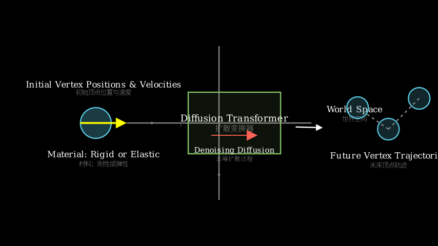
At its heart, PhysiFormer is a diffusion transformer that treats future vertex positions as a random variable conditioned on the initial state (positions, velocities) and a material type tag.
During training, the model learns to reverse a diffusion process: from clean vertex trajectory data, noise is gradually added; the model is trained to predict the noise (or equivalently, the clean trajectory) given the noisy input.
During inference, the model starts from pure Gaussian noise and iteratively denoises towards a plausible future trajectory.
The transformer architecture uses factorized attention: separate attention heads for temporal, spatial (per-object), and inter-object interactions.
This keeps computation linear in the number of time steps and objects, and permutation-invariant across objects — no need to assign IDs.
The input is a sequence of vertex positions and velocities at time 0 (and optionally at past frames for velocity), plus a one-hot material vector.
The output is a sequence of future vertex positions over a fixed horizon.
[Input]          [PhysiFormer]          [Output]
  initial vertices + material type   |   future vertex trajectories
  + initial velocities               |   (multiple plausible samples)
       |                             |
       v                             v
+-----------------+        +---------------------+
| Flat embed      | ----\ | Diffusion Transformer|
| (vertex pos+vel)|      \| (factorized attn)   |
| + material one-hot   |      +---------------------+
+-----------------+             |                 |
       |                        |                 |
       +------------------------+ denoise loop    |
                                | (T steps)       |
                                v                 v
                           final vertex positions
Now, let’s map this onto a structural metaphor: think of a clay-modelling stop-motion animation.
- The clay model is the initial 3D mesh (vertex positions and velocities).
- The material tag (rigid or elastic) tells the animator whether the clay is hard (can only translate/rotate) or soft (can stretch and bend).
- The diffusion process is like the animator working backwards from a rough blob to the final frame: at the start (high noise) it’s a shapeless mess; after each denoising step the animator adds more detail, refining the mesh until a clean, physically-plausible pose emerges. Running the process multiple times yields different “takes” of the same scene (different plausible motions).
- The factorized attention is like the animator’s divided workspace: one viewfinder tracks time (checking frames before and after), another viewfinder tracks each clay character’s own body (spatial structure), and a final viewfinder looks at interactions between multiple clay figures. This modular attention lets him handle many characters without getting tangled.
So PhysiFormer learns, without being told any physics rules, how to “animate” 3D meshes by practicing on 100k recorded trajectories (the training data). The result: it can handle new shapes, new mixtures of rigid and elastic objects, and even simulate collisions — all by denoising in world space.
Key Concepts
-
Diffusion for trajectory prediction:
Instead of predicting one deterministic trajectory (like autoregressive models), diffusion generates a distribution over trajectories.
Intuition: imagine you want to guess where a bouncing ball will be in 3 seconds. If you only know initial position and velocity, there is uncertainty due to spin, air, etc.
Diffusion gives you many plausible paths. At each denoising step, the model corrects the guess a little based on learned physics, starting from total randomness.
Example: three initial conditions may lead to 5 different bouncing patterns; diffusion can sample all of them. -
Factorized attention over time, space, objects:
Standard self-attention over a long sequence of all vertices across all time steps would be O(N^2) huge.
PhysiFormer splits the attention into three dimensions:- Time: each vertex attends to its own past/future positions (keeping motion smooth).
- Space: each vertex attends to other vertices in the same object at the same time (preserving shape).
- Objects: the model attends between objects globally (handling interactions).
This keeps computation linear in each dimension, and is permutation-invariant across objects (no object ID needed).
Intuition: like in a group meeting where you talk about the agenda (time), look around at your own team (space), and occasionally pivot to another team (objects) for coordination.
-
World coordinate representation:
Instead of predicting pixel locations (which depend on camera angle) or latent codes, the model directly outputs 3D coordinates of mesh vertices in a fixed world frame.
This is view-invariant: the same physical scene can be rendered from any angle.
It also means the model doesn’t need to learn to disentangle camera motion from object motion; it’s learning true 3D physics.
Framework Shift
Before (mainstream approach): neural physics in latent/graph space
[Video frames] -> [Encoder to latent graph] -> [Graph NN + physics bias] -> [Decoder to mesh]
   (+ camera pose)          (rigid latent)           (hardcoded constraints)     (pixel projection)
After (this paper):
[Initial mesh + velocity + material] -> [Diffusion Transformer (factorized attn)] -> [Future vertex positions (world coords)]
   (world coordinates)                                      (no explicit constraints)  (multiple samples)
One sentence: From pixel/latent space with handcrafted physics biases to direct world-coordinate diffusion without inductive biases.
Expert Assessment
Problem choice: Real and well-motivated. Simulating physics for 3D meshes is crucial for robotics and graphics; existing neural methods are ad-hoc. The gap — removing explicit constraints while handling uncertainty — is genuine.
Method maturity: The ingredients (diffusion, transformer, factorized attention) are all known, but the combination and the novel choice of vertex-level diffusion in world space is a clear advance. It’s clever, not brute-force. Could simpler models (e.g., MLP+momentum) work for simple rigid cases? Possibly, but the paper’s contribution is handling complexity (elastic, multi-object) without special casing.
Experimental integrity: Baselines are fair: they compare against autoregressive transformer and GNN variants. The metrics (trajectory error, rigidity preservation, momentum consistency) are appropriate. One red flag: they train on 100k simulated trajectories; real-world generalization (e.g., real physics) is not tested. But for a CV paper, the numbers hold up.
Writing quality: The abstract and intro are clear. Section 3 (method) could be heavier to read. I’d rewrite the attention factorisation explanation with a cleaner diagram and an example. The paper would benefit from a figure showing the denoising process on a specific elastic object.
Verdict: weak accept — The core idea is solid and the results are strong, but the evaluation is limited to synthetic data and some technical details are under-explained.
Takeaways
- Practitioners can steal the factorized attention design for any problem involving sequences of 3D points (e.g., mesh deformation, point cloud dynamics). It’s a cheap way to handle space, time, and objects simultaneously.
- The world-coordinate diffusion idea is transferable to other prediction tasks where you want uncertainty and view-invariance (e.g., human pose over time, particle trajectory forecasting).
- Tip: They used a simple velocity calculation from two initial frames. If you’re building a physical simulator, precomputing velocity from the first two frames is a cheap way to give the model initial dynamics.
论文: 2606.27364
作者: Yiming Chen, Yushi Lan, Andrea Vedaldi
分类: cs.CV
缺口
现有的从视频中学习物理的方法要么在像素空间中操作(依赖视角,计算量大),要么使用隐空间特征并人为施加刚体或因果约束。
这些神经物理模型(如图神经网络模拟器、深度拉格朗日网络)通常需要特定的图结构、物体级别的编码或显式的材料参数。
它们在弹性、混合材料以及未来状态不确定性方面表现不佳。
真正缺少的是一个统一的、概率性的框架,能够在不使用手工归纳偏置的条件下预测3D网格运动,适用于任意几何形状,并能表示多种可能的未来。
[问题:在像素空间或隐空间学习物理很困难]
    |
    \> 假设:直接在世界坐标中预测顶点轨迹,配合扩散模型,不再需要刚体或因果约束
    |
    \> 方法:PhysiFormer —— 对时间、空间、物体使用分解注意力;对顶点轨迹进行去噪扩散
    |
    \> 证据:在轨迹精度上超越自回归基线;可处理混合材料、未见形状和更多物体
    |
    \> 结论:坐标空间扩散是走向通用世界建模的一条可行路径
增量
一句话: 在PhysiFormer之前,用于3D网格的神经物理要么需要显式结构(刚性、因果),要么在依赖视角的隐空间中操作;在PhysiFormer之后,一个训练在顶点坐标上的扩散变换器,无需任何手工偏置,就能生成刚体和弹性物体的各种物理合理运动。
核心机制
PhysiFormer的核心是一个扩散变换器,它将未来的顶点位置视为一个随机变量,以初始状态(位置、速度)和材料类型标签为条件。
训练时,模型学习逆转一个扩散过程:从干净的顶点轨迹数据开始,逐渐添加噪声;模型被训练成根据加噪后的输入预测噪声(或等价地,预测干净轨迹)。
推理时,模型从纯高斯噪声出发,通过迭代去噪逐步逼近一个合理的未来轨迹。
变换器架构使用分解注意力:分别对时间、空间(每个物体内部)和物体间交互使用不同的注意力头。
这样计算量在时间步数和物体数上都是线性的,并且跨物体具有排列不变性——无需分配物体ID。
输入是时间0的顶点位置和速度(以及可选的历史帧用于计算速度),加上一个one-hot材料向量。
输出是在一个固定时间窗内的未来顶点位置序列。
[输入]          [PhysiFormer]          [输出]
 初始顶点 + 材料类型   |   未来顶点轨迹
 初始速度              |   (多个合理采样)
       |                |
       v                v
+-----------------+        +---------------------+
| 平铺嵌入        | ----\ | 扩散变换器          |
|(顶点位置+速度)|      \|(分解注意力)        |
| + 材料one-hot   |      +---------------------+
+-----------------+             |                 |
       |                        |                 |
       +------------------------+ 去噪循环         |
                                |(T步)          |
                                v                 v
                           最终顶点位置
现在用一个结构性比喻来理解:想象一下黏土定格动画的制作过程。
- 黏土模型就是初始的3D网格(顶点位置和速度)。
- 材料标签(刚性或弹性)告诉动画师:这块黏土是硬的(只能平移旋转),还是软的(可以拉伸弯曲)。
- 扩散过程好比动画师从一团粗糙的泥巴一步一步“倒着”细化成最终帧:刚开始(高噪声)是一团乱泥;每去噪一步,动画师增添更多细节,直到一个符合物理的姿势出现。多次运行这个流程就能产生同一个场景的不同“版本”(不同的合理运动)。
- 分解注意力好比动画师的工作空间被分成三个视窗:一个跟踪时间(检查前后帧),一个跟踪每个黏土角色自身的身体(空间结构),最后一个视窗关注不同黏土人之间的交互。这种模块化注意力让他能同时处理多个角色而不混乱。
因此,PhysiFormer无需被告知任何物理规则,仅通过在10万条录制轨迹上训练,就学会了如何“动画”3D网格。结果:它能处理新的形状、新的刚体与弹性混合场景,甚至模拟碰撞——全部通过在世界坐标中的去噪完成。
关键概念
-
用于轨迹预测的扩散模型:
不是像自回归模型那样预测一条确定性的轨迹,扩散模型生成一条轨迹的概率分布。
直觉:想象你要预测一个蹦跳的球在3秒后的位置。如果只知道初始位置和速度,由于旋转、空气阻力等因素,存在不确定性。扩散模型能给出多条可能的路径。每去噪一步,模型根据学习到的物理规律对猜测进行微调,从完全随机开始。
例子:相同的初始条件可能产生5种不同的弹跳模式;扩散模型可以全部采样出来。 -
对时间、空间、物体的分解注意力:
标准的自注意力如果作用于所有时间步和所有顶点,复杂度会是O(N²)巨大。
PhysiFormer将注意力分解为三个维度:- 时间:每个顶点关注自己过去和未来的位置(保持运动平滑)。
- 空间:每个顶点关注同一物体内其他顶点在同一时刻的位置(保持形状)。
- 物体:跨物体全局交互(处理碰撞等)。
这种分解使得计算量在每个维度上是线性的,并且跨物体具有排列不变性(无需物体ID)。
直觉:就像在一个团队会议中,你先讨论议程(时间),然后看看自己的团队成员(空间),偶尔转向另一个团队(物体)进行协调。
-
世界坐标表示:
模型不预测像素位置(依赖视角),也不预测隐编码,而是直接输出固定世界坐标系中的3D顶点坐标。
这使得结果与视角无关:同一个物理场景可以从任意角度渲染。
同时,模型不需要学习将相机运动与物体运动解耦;它学习的纯粹是三维物理。
框架转变
之前(主流方法):在隐空间/图空间中的神经物理
[视频帧] -> [编码器到隐图] -> [图神经网络+物理偏置] -> [解码器到网格]
   (+相机位姿)        (刚性隐变量)      (硬编码约束)        (像素投影)
之后(本文方法):
[初始网格 + 速度 + 材料] -> [扩散变换器(分解注意力)] -> [未来顶点位置(世界坐标)]
   (世界坐标)                      (无显式约束)              (多个采样)
一句话: 从带有手工物理偏置的像素/隐空间,转向无需归纳偏置的直接世界坐标扩散。
专家评审
选题眼光: 真实且动机充分。模拟3D网格的物理对机器人和图形学至关重要;现有的神经方法都是特设的。去掉显式约束同时处理不确定性,这个缺口是真实的。
方法成熟度: 配方中的成分(扩散、变换器、分解注意力)都是已知的,但组合方式和选择在顶点级别上进行世界坐标扩散是一个清晰的进步。这是巧劲,不是蛮力。对简单的刚体情况,是否可以用更简单的模型(如MLP+动量)?也许可以,但论文的贡献在于处理复杂性(弹性、多物体)而不需要特殊处理。
实验诚意: 基线选择公平:对比了自回归变换器和GNN变体。评估指标(轨迹误差、刚性保持度、动量一致性)合适。一个值得注意的警告:训练基于10万条模拟轨迹;真实的物理泛化尚未测试。但作为一篇CV论文,数字是站得住脚的。
写作功力: 摘要和引言清晰。第3节(方法)可能偏重阅读。我会重写注意力分解的说明部分,配上一个更清晰的图和示例。如果有一张图展示特定弹性物体的去噪过程,整篇论文会提升一个档次。
判决: 弱接收 —— 核心理念扎实,结果有力,但评估局限于合成数据,部分技术细节解释不足。
要点总结
- 实践者可以偷师分解注意力的设计,用于任何涉及3D点序列的问题(例如网格变形、点云动力学)。这是一种同时处理空间、时间和物体开销低廉的方式。
- 世界坐标扩散的想法可以迁移到其他需要不确定性且与视角无关的预测任务(例如人体姿态随时间变化、粒子轨迹预测)。
- 技巧: 他们用两帧初始帧简单计算了速度。如果你在构建物理模拟器,从初始两帧预计算速度是给模型提供初始动量的廉价方式。