Neural Field Thermal Tomography: Hard Physics Constraints Meet Continuous 3D Reconstruction

Paper: 2603.11045 Authors: Tao Zhong, Yixun Hu, Dongzhe Zheng, Aditya Sood, Christine Allen-Blanchette Categories: cs.LG, cond-mat.mtrl-sci, cs.AI, cs.CV, physics.ins-det

The Gap

Industrial non-destructive testing needs to find subsurface defects without cutting things open. Thermography does this by heating a surface and watching how temperature evolves—defects change heat flow patterns. But existing approaches hit two walls.

Traditional thermography treats each pixel independently, solving 1D heat equations that ignore lateral diffusion. This works for simple cases but fails when heat spreads sideways around defects. Physics-Informed Neural Networks (PINNs) tried to fix this by learning 3D solutions, but they use soft constraints—the network “tries” to satisfy physics laws through loss terms. In transient diffusion problems, gradients become stiff (rapid changes in time, slow in space), and soft constraints collapse. The network can’t balance fitting data and obeying physics.

The gap: we need 3D reconstruction that respects thermodynamics as hard constraints, not suggestions, while remaining memory-efficient enough for high-resolution tomography.

Problem: Find subsurface defects from surface temperature
    |
    v
Assumption: Heat diffusion obeys known PDEs,
            but material properties (diffusivity) are unknown
    |
    v
Method: Parameterize 3D diffusivity as neural field,
        optimize via differentiable physics solver
    |
    v
Evidence: Synthetic experiments show improved
          defect localization vs baselines
    |
    v
Conclusion: Hard constraints + continuous representation
            beats soft constraints for inverse diffusion

The Increment

One sentence: Before NeFTY, you chose between 1D approximations that ignore physics or 3D PINNs that can’t enforce it—now you get 3D reconstruction with thermodynamics as hard constraints through differentiable solvers.

Core Mechanism

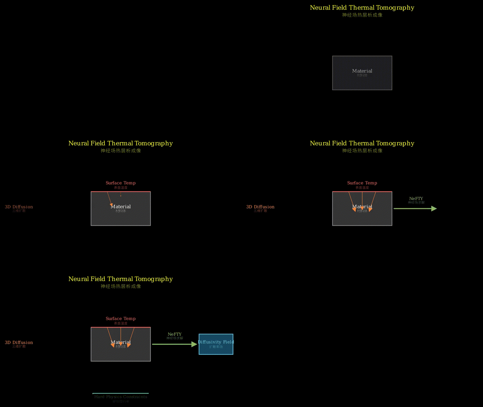
NeFTY has three components working in sequence. First, a neural field (coordinate-based MLP) represents 3D thermal diffusivity as a continuous function—query any (x,y,z) coordinate, get a diffusivity value. Second, a differentiable finite-difference solver takes this diffusivity field and simulates forward heat diffusion, producing predicted surface temperatures. Third, an optimizer adjusts neural field parameters to minimize the gap between predicted and measured temperatures.

The key is “discretize-then-optimize”: discretize the continuous neural field onto a grid, solve the discrete heat equation exactly (hard constraint), then backpropagate through the solver to update the neural field. This contrasts with PINNs’ “optimize-then-discretize” where the network directly outputs temperatures and physics appears only as a soft loss term.

Data flows like this: surface measurements → loss computation → gradients through solver → neural field parameter updates → refined diffusivity field → better forward predictions. The solver acts as a differentiable physics engine, converting material properties into observable temperatures while guaranteeing thermodynamic consistency at every step.

Input: Surface temperature measurements T_surface(x,y,t)
   |
   v
[Neural Field: MLP]  <--- Parameters theta
   |                       (optimized)
   | query (x,y,z)
   v
Diffusivity field: k(x,y,z)
   |
   | discretize to grid
   v
[Differentiable PDE Solver]
   | forward: k(x,y,z) -> T(x,y,z,t)
   | backward: dL/dT -> dL/dk -> dL/dtheta
   v
Predicted T_surface(x,y,t)
   |
   v
Loss: ||T_pred - T_measured||^2
   |
   v
Gradient descent on theta

Think of it like sculpting with X-rays. You have a block of clay (the 3D volume) but can only see its shadow (surface temperatures). Traditional methods carve each column independently, ignoring how removing clay from one column affects neighbors. PINNs try to imagine the whole sculpture at once, but their mental model is fuzzy—they “kind of” respect how clay behaves. NeFTY instead uses a physics simulator as a strict teacher: propose a sculpture (diffusivity field), the simulator shows you exactly what shadow it would cast (surface temperatures via heat equation), compare to the real shadow, then adjust your sculpture. The neural field is your sculpting tool (continuous, smooth adjustments), the differentiable solver is your X-ray machine (shows consequences of every change), and optimization is your iterative refinement process.

Key Concepts

• Neural Fields: Instead of storing diffusivity values in a 3D array (memory explodes at high resolution), represent it as a function approximated by a neural network. Feed in coordinates (x,y,z), get out diffusivity k. The network learns a compressed, continuous representation. Imagine describing a mountain not by listing every rock’s position, but by learning a formula that generates elevation at any point. You can query infinite resolution from finite parameters, and the function is naturally smooth (networks interpolate well). For thermal tomography, this means representing complex defect geometries without pre-committing to grid resolution.

• Differentiable Physics Solver: A numerical PDE solver (finite differences, finite elements) that computes gradients. Normally, solvers are black boxes: input → output. Making them differentiable means tracking how output changes with input, enabling gradient-based optimization. The trick: treat the solver as a computational graph. Each discretization step (spatial derivatives, time stepping) becomes a differentiable operation. Backpropagation flows through the entire simulation. This enforces physics as a hard constraint—the solver always produces physically valid solutions—while still allowing optimization. It’s like having a physics engine that not only simulates but also tells you “if you changed this parameter slightly, here’s exactly how the outcome would shift.”

• Discretize-then-Optimize vs Optimize-then-Discretize: PINNs optimize-then-discretize: the network directly outputs field values, physics appears as a loss term (soft constraint), then you discretize for evaluation. NeFTY discretizes-then-optimizes: sample the neural field onto a grid, solve the discrete PDE exactly (hard constraint), then optimize the continuous field parameters. The difference matters for stiff problems. In transient diffusion, time derivatives are large, spatial derivatives small. Soft constraints struggle to balance these scales—the network finds shortcuts that approximately satisfy physics but miss fine details. Hard constraints guarantee correctness at every optimization step, avoiding gradient pathologies. It’s the difference between “try to obey traffic laws” (soft) versus “physically cannot break them” (hard).

Framework Shift

Before (PINNs):                    After (NeFTY):
                                   
Neural Net                         Neural Field (continuous)
    |                                  |
    v                                  v discretize
Predict T(x,y,z,t)                 Diffusivity k(x,y,z)
    |                                  |
    v                                  v
Loss = Data + Physics              Differentiable Solver
       (soft constraint)               | (hard constraint)
                                       v
                                   Predict T(x,y,z,t)
                                       |
                                       v
                                   Loss = Data only

From soft-constrained direct prediction to hard-constrained inverse modeling, the core shift is treating physics as a non-negotiable simulator rather than a regularization term.

Expert Assessment

Problem choice: Real gap. Non-destructive evaluation is a billion-dollar industry (aerospace, manufacturing), and current thermography methods genuinely struggle with 3D reconstruction. The PINN failure mode (gradient stiffness in transient diffusion) is well-documented. This isn’t manufactured—it’s a known pain point where existing ML approaches underdeliver.

Method maturity: Clever assembly of existing pieces. Neural fields (NeRF-style) and differentiable physics solvers both exist; the contribution is recognizing their combination solves the PINN failure mode. The “discretize-then-optimize” framing is conceptually clean but not deeply novel—it’s standard in PDE-constrained optimization, just newly applied to neural implicit representations. No simpler approach is obviously overlooked, though one wonders if classical regularized inversion with learned priors might compete.

Experimental integrity: Red flag: only synthetic data. No real thermal camera experiments, no comparison to actual industrial thermography systems. Baselines are reasonable (traditional 1D methods, PINNs) but the paper doesn’t test against domain-specific methods like pulsed thermography with advanced signal processing. The synthetic setup lets them control ground truth, but it sidesteps noise, calibration, and model mismatch issues that plague real inverse problems. Numbers look good but need real-world validation.

Writing quality: Abstract is dense—packs too many concepts (neural fields, differentiable solvers, spectral bias, gradient stiffness) without breathing room. The “discretize-then-optimize” framing is buried; it should lead. Section on why PINNs fail could be expanded—gradient stiffness is mentioned but not explained. If they rewrote the introduction to build intuition for the hard-constraint advantage before diving into technical details, the paper would land better.

Verdict: weak accept — Solid contribution to an applied problem with clear motivation, but experimental validation is incomplete and the method is more engineering than algorithmic novelty.

Takeaways

Practitioners working on inverse problems can steal the “differentiable simulator as hard constraint” pattern. If you’re using neural networks to solve PDEs and hitting optimization issues, ask: am I treating physics as a loss term (soft) or as a forward model (hard)? Wrapping a classical solver in autodiff often beats end-to-end learning when you know the governing equations. The neural field parameterization is also transferable—anytime you need continuous 3D representations (medical imaging, geophysics, materials science), coordinate-based MLPs give you resolution-independent, memory-efficient fields. Finally, the paper’s framing of “spectral bias” (networks struggle with high-frequency details) as solvable via hard constraints is worth remembering: sometimes the fix isn’t better architectures but better problem formulation.