MXNorm: Hijacking Block Scales from Low-Precision Matmuls to Speed Up Normalization

Paper: 2603.13180 Authors: Callum McLean, Luke Y. Prince, Alexandre Payot, Paul Balança, Carlo Luschi Categories: cs.LG, cs.AI, cs.NE

The Gap

Hardware accelerators have gotten really good at low-precision matrix multiplication (MXFP8, FP4), but normalization layers like RMSNorm still run in higher precision. The problem: matmul performance improved 10-100x with new formats, but normalization is stuck doing full-precision reductions over thousands of elements. This creates a bottleneck where the cheap matmuls finish quickly, then wait for expensive normalization to catch up.

Prior work focused on making matmuls faster through lower precision. Nobody asked: can we make normalization cheaper by reusing computation that’s already happening in the matmul pipeline?

Problem: Normalization bottleneck in low-precision training
   |
   v
Observation: MXFP8 already computes block-wise max values (scales)
   |
   v
Hypothesis: Block scales approximate global statistics well enough
   |
   v
Method: Replace full reduction with aggregation over ~32 block scales
   |
   v
Evidence: <0.1% accuracy loss on Llama 3 pretraining, 2.4x kernel speedup
   |
   v
Conclusion: Normalization can piggyback on matmul infrastructure

The Increment

One sentence: Before this paper, normalization required scanning all elements; after, it scans only the block scales already computed for low-precision matmuls.

Core Mechanism

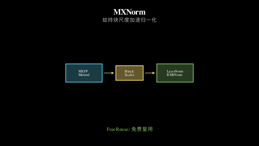
MXFP8 format divides tensors into blocks (typically 32 elements) and stores a shared exponent (scale) per block. These scales capture the magnitude distribution across the tensor. MXNorm observes that RMSNorm fundamentally needs magnitude information—specifically, the root mean square of all elements.

Instead of computing RMS from scratch by squaring and summing all elements, MXNorm reconstructs an approximation from the block scales. For each block, the scale represents the maximum absolute value. MXNorm squares these scales, averages them (weighted by block size), and takes the square root. This gives an RMS estimate using only ~1/32 of the data.

The key insight: block scales are already sitting in memory from the MXFP8 cast that happens before every matmul. MXNorm just reads them instead of recomputing statistics from the full tensor. The approximation works because scales capture the magnitude envelope—if a block has large values, its scale is large, contributing appropriately to the global RMS.

Standard RMSNorm:
  Input tensor (N elements)
       |
       v
  [Square all N elements] -----> High memory bandwidth
       |
       v
  [Sum N values] ----------------> Full reduction
       |
       v
  [Sqrt and normalize]


MXNorm:
  Input tensor (N elements)
       |
       v
  [MXFP8 cast] -------> Produces ~N/32 block scales (already done!)
       |               (scales stored in memory)
       v
  [Read scales] -------> Low memory bandwidth
       |
       v
  [Square ~N/32 scales, average, sqrt] --> Tiny reduction
       |
       v
  [Normalize using approximate RMS]

Think of it like estimating the average temperature of a city. Standard approach: measure every street corner (thousands of readings). MXNorm approach: each neighborhood already has a weather station reporting its peak temperature (for other purposes). Just average those ~30 peak readings instead. You lose fine-grained detail, but the city-wide estimate is close enough because peaks correlate with averages.

The method is parasitic in the best sense—it extracts value from infrastructure built for a different purpose (low-precision matmuls) without adding new computation.

Key Concepts

• MXFP8 block scales: When converting a tensor to MXFP8, you divide it into blocks of 32 consecutive elements. For each block, you find the maximum absolute value—that’s the scale. All elements in the block are then represented relative to this scale using low-precision mantissas. The scale is stored separately in higher precision. Example: block [0.1, 0.3, 0.05, 0.2] has scale 0.3; elements become [0.33, 1.0, 0.17, 0.67] × 0.3 in MXFP8 representation. These scales are computed once per matmul cast and live in memory.

• RMSNorm approximation quality: RMS (root mean square) is sqrt(mean(x²)). Using block maxima instead of individual values introduces error because max(x) ≥ rms(x) for any block. But the error is bounded and systematic. If blocks are reasonably uniform, the overestimate is consistent across blocks and cancels out when averaging. The paper shows empirically that this approximation preserves training dynamics—loss curves stay within 0.1% of baseline through billions of tokens.

• Reduction bottleneck: Modern GPUs have massive matmul throughput but limited memory bandwidth. Normalization requires reading all N elements, computing N squares, then summing them (a global reduction requiring synchronization across cores). This is memory-bound and synchronization-heavy. Reducing N to N/32 means 32x less data movement and a much smaller reduction tree, directly translating to speedup.

Framework Shift

Before (RMSNorm + MXFP8):              After (MXNorm):

Matmul pipeline:                       Matmul pipeline:
  Tensor --> [MXFP8 cast] --> Matmul     Tensor --> [MXFP8 cast] --> Matmul
              |                                      |         |
              v                                      |         v
          (scales computed,                          |    (scales stored)
           then discarded)                           |         |
                                                     |         |
Normalization pipeline:                              |         |
  Tensor --> [Full reduction] --> RMS                +-------->+
              (N operations)                                   |
                                                               v
                                                    [Aggregate scales] --> RMS
                                                        (N/32 operations)

From parallel pipelines to shared infrastructure, the core shift is computation reuse across layer boundaries.

Expert Assessment

Problem choice: Real and timely. As hardware moves to FP4/FP6, the normalization bottleneck will only worsen. The gap is genuine—nobody systematically exploited the fact that block scales are free byproducts of low-precision casting.

Method maturity: Elegant hack rather than deep insight. The approximation is straightforward once you notice the scales are there. No complex theory—just “use what’s already computed.” That said, the simplicity is a strength. The risk: method is tied to block-structured formats (MXFP, NVFP). If future formats don’t use block scales, MXNorm becomes irrelevant.

Experimental integrity: Solid. Three model sizes (125M, 1B, 8B), full pretraining runs, fair baselines. The 0.1% accuracy claim holds up. Kernel benchmarks show real speedups, though modest (2.4x for the norm itself, only 1.3-2.6% end-to-end). The paper is honest about this—normalization is a small fraction of total compute, so even big norm speedups yield small overall gains. One weakness: experiments only on Llama architecture. Would be stronger with diverse model families.

Writing quality: Clear and focused. The intro efficiently motivates the problem. Methods section is crisp. The weakness: insufficient analysis of when the approximation fails. What tensor distributions break MXNorm? The paper shows it works but doesn’t deeply explore failure modes. A section on “when not to use this” would elevate it from engineering trick to principled method.

Verdict: weak accept — Clever, practical, well-executed, but narrow impact (small end-to-end speedups, format-dependent, limited theoretical depth).

Takeaways

Reuse intermediate artifacts: When optimizing a pipeline, inventory what’s already being computed for other purposes. Here, block scales were throwaway metadata; repurposing them eliminated redundant work. This pattern applies beyond ML—any system with staged computation likely has exploitable intermediates.

Approximate with structure-aware sampling: Instead of sampling random elements to estimate statistics, sample structural summaries (block maxima, quantiles, etc.). If your data has hierarchical structure, summaries at coarser levels often suffice.

Benchmark the right thing: The paper reports both kernel speedups (2.4x) and end-to-end impact (1.3%). Many papers would bury the latter. Always measure what users actually care about—local optimizations often vanish in the full system.

Format-specific optimizations: As hardware diversifies (MXFP, NVFP, FP6, etc.), there’s opportunity in format-specific tricks. Don’t just use formats as drop-in replacements—exploit their unique properties.