Mixture-of-Depths Attention: Letting Deep Layers Remember Shallow Insights

Paper: 2603.15619 Authors: Lianghui Zhu, Yuxin Fang, Bencheng Liao, Shijie Wang, Tianheng Cheng, Zilong Huang, Chen Chen, Lai Wei, Yutao Zeng, Ya Wang Categories: cs.CL, cs.AI

The Gap

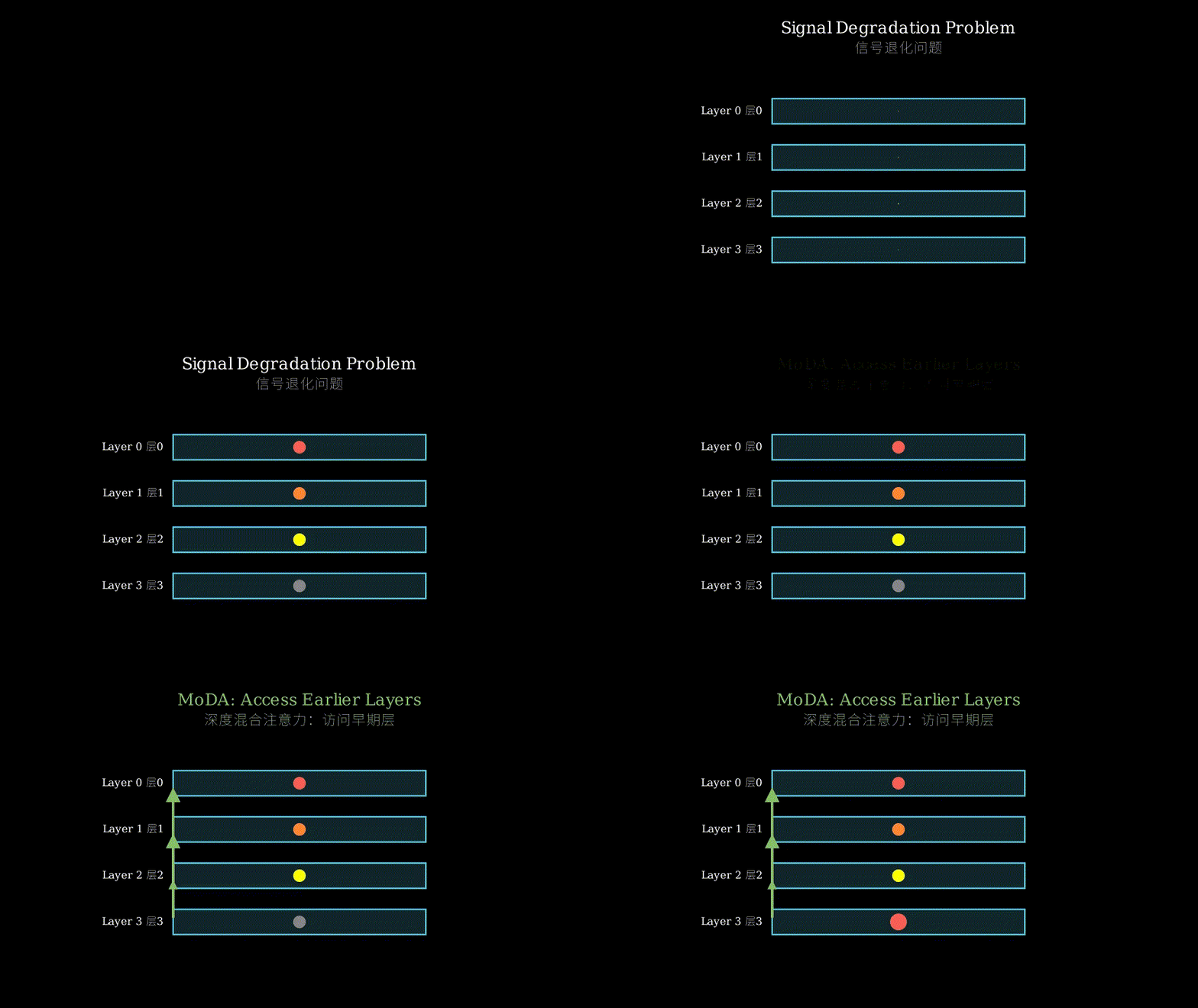
Deep networks are supposed to get smarter with more layers. But there’s a dirty secret: as LLMs grow deeper (50+ layers), useful features formed in shallow layers get progressively washed out by repeated residual additions. By layer 40, the sharp insights from layer 5 are buried under 35 layers of incremental updates. Standard attention mechanisms only look at the current layer’s representations—they can’t reach back to recover those early, crisp features.

Prior work scaled depth aggressively (GPT-3: 96 layers, PaLM: 118 layers) but treated each layer as a pure function of the previous one. The residual connection helps gradient flow, but it doesn’t prevent information dilution. Some approaches tried skip connections or dense connections (DenseNet-style), but these either explode memory or don’t integrate cleanly with transformer attention.

Problem: Signal Degradation
    |
    v
Assumption: Early layers form useful features
            that get diluted by residual updates
    |
    v
Method: Let attention heads access KV pairs
        from both current AND previous layers
    |
    v
Evidence: 0.2 perplexity drop, 2.11% task improvement
          with 3.7% FLOPs overhead (1.5B params)
    |
    v
Conclusion: Depth-aware attention preserves
            shallow features in deep networks

The Increment

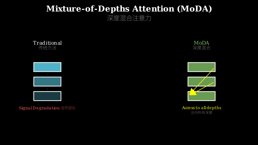
One sentence: Before MoDA, attention was layer-local (only current representations); after MoDA, attention is depth-aware (can query earlier layers directly).

Core Mechanism

Standard attention computes queries, keys, and values from the current layer’s hidden states. MoDA extends this: each attention head now has access to two pools of KV pairs. The first pool is the usual sequence KV pairs from the current layer (length N). The second pool is depth KV pairs—a curated selection of KV pairs from all preceding layers (length M, where M is typically much smaller than N).

When computing attention, the query vector attends to the concatenation of both pools. This means a head in layer 40 can directly attend to features from layer 5 without them having to survive 35 residual additions. The depth KV pairs are selected via a learned gating mechanism that picks the most informative representations from each earlier layer.

The hardware challenge: accessing KV pairs from multiple layers creates non-contiguous memory patterns that kill GPU efficiency. The authors solve this with a clever algorithm that reorganizes memory access to maintain spatial locality, achieving 97.3% of FlashAttention-2’s speed even at 64K sequence length.

Standard Attention (Layer L):
    Q, K, V = Linear(H_L)
    Output = Attention(Q, K, V)  [attends to N tokens]

MoDA (Layer L):
    Q = Linear(H_L)
    K_seq, V_seq = Linear(H_L)           [N sequence KVs]
    K_depth, V_depth = Select(H_1...H_L-1) [M depth KVs]
    K_all = Concat(K_seq, K_depth)       [N+M total]
    V_all = Concat(V_seq, V_depth)
    Output = Attention(Q, K_all, V_all)

Think of it like a research library with multiple floors. Standard attention is like being on floor 40 and only being able to reference books on that floor—you have to trust that important information from floor 5 made it up through the elevator (residual connection). MoDA installs a pneumatic tube system: you can still browse floor 40’s books, but you can also send a request down to any lower floor and get specific books sent up directly. The tube system (depth KV selection) is smart—it doesn’t send every book from every floor (that would overwhelm you), just the most relevant ones based on what you’re researching (learned gating). The pneumatic tubes are engineered for speed (hardware-efficient algorithm), so getting books from floor 5 is nearly as fast as grabbing one from the shelf next to you.

Key Concepts

• Signal Degradation: Imagine you’re playing telephone with 50 people. Person 1 says “The red fox jumped over the lazy brown dog.” By person 50, it’s “Something about animals.” That’s signal degradation. In deep networks, each layer adds a small update via residual connection: H_L = H_{L-1} + F(H_{L-1}). After 50 additions, the original H_1 is diluted—its signal-to-noise ratio drops. Features that were sharp and distinct in layer 5 become fuzzy and mixed with everything else by layer 50. MoDA fights this by letting layer 50 directly access layer 5’s representation, bypassing the telephone game.

• Depth KV Pairs: In standard attention, you have N tokens in your sequence, so you have N key-value pairs. MoDA adds a second dimension: depth. For a model with L layers, you could theoretically have L×N KV pairs (every token at every layer). But that’s computationally insane. Instead, MoDA selects M representative KV pairs from all previous layers (M << L×N). Think of it as taking a core sample through geological strata—you don’t need every grain of sand from every layer, just representative samples that preserve the essential information from each depth.

• Hardware-Efficient Memory Access: GPUs are fast when you read memory sequentially (like reading a book page by page). They’re slow when you jump around (like reading page 5, then page 203, then page 47). Accessing KV pairs from multiple layers creates a “random access” pattern—layer 40’s KVs are in one memory region, layer 5’s are far away. The authors reorganize how KV pairs are stored in memory so that the depth KVs you need are clustered together, turning random access into sequential access. It’s like reorganizing your bookshelf so that all the books you need for your current project are on one shelf, even if they’re from different topics.

Framework Shift

Before (Standard Transformer):        After (MoDA):

Layer 40: [H_40] ---> Attn(H_40)     Layer 40: [H_40] ---> Attn(H_40 + samples from H_1...H_39)
            |                                      |
Layer 39: [H_39] ---> Attn(H_39)     Layer 39: [H_39] ---> Attn(H_39 + samples from H_1...H_38)
            |                                      |
   ...      |                            ...       |
            |                                      |
Layer 5:  [H_5]  ---> Attn(H_5)      Layer 5:  [H_5]  ---> Attn(H_5 + samples from H_1...H_4)
            |                                      |
Layer 1:  [H_1]  ---> Attn(H_1)      Layer 1:  [H_1]  ---> Attn(H_1)

Information flow: Sequential          Information flow: Sequential + Direct shortcuts
(each layer only sees previous)       (each layer sees previous + selected earlier layers)

From sequential information flow to multi-scale information flow, the core shift is enabling direct access to earlier representations without forcing them through the residual bottleneck.

Expert Assessment

Problem choice: This is a real gap, not manufactured. Signal degradation in deep networks is well-documented (see residual network literature, highway networks). The problem becomes acute as models scale to 100+ layers. The authors are addressing a genuine bottleneck in depth scaling, which is timely given the push toward deeper models.

Method maturity: This is clever but not revolutionary. The core idea—let attention access multiple layers—is straightforward. The real contribution is making it hardware-efficient. The learned gating for selecting depth KVs is sensible but not deeply explored (how sensitive is it to initialization? does it learn interpretable patterns?). I’d like to see ablations on the selection mechanism. The post-norm finding (MoDA + post-norm > MoDA + pre-norm) is interesting but under-explained—why does this interaction exist?

Experimental integrity: Baselines are fair (standard transformer, other depth-scaling approaches). The 1.5B parameter scale is reasonable for exploration but not conclusive—does this hold at 7B? 70B? The 0.2 perplexity improvement is modest but consistent across 10 benchmarks, which is reassuring. The 2.11% downstream task improvement is more impressive. The 3.7% FLOPs overhead is honest reporting (many papers hide computational costs). One red flag: no comparison with mixture-of-experts (MoE), which also adds conditional computation. How does MoDA compare to MoE in the efficiency-performance tradeoff?

Writing quality: The paper is clear but front-loads too much motivation. The “signal degradation” framing is good, but they spend two pages on it when one would suffice. The hardware efficiency section is well-written—this is where the real engineering work lives. The ablation studies are adequate but not exhaustive. If I were rewriting, I’d expand the analysis of what the depth KV selection learns (visualizations, interpretability) and cut the redundant motivation paragraphs.

Verdict: Weak accept—solid incremental work that addresses a real problem with a practical solution, but not a paradigm shift.

Takeaways

For practitioners: If you’re training deep models (30+ layers) and hitting diminishing returns, MoDA is worth trying. The 3.7% FLOPs overhead is negligible, and the 2% task improvement could matter for production systems. The hardware-efficient implementation means you can actually deploy this without rewriting your training infrastructure.

For researchers: The core idea—attention across layers, not just tokens—generalizes beyond transformers. You could apply this to any deep architecture where information dilution is a problem (ResNets, U-Nets, etc.). The learned gating mechanism for selecting which earlier representations to preserve is under-explored and could be a research direction on its own.

Specific technique to steal: The memory reorganization trick for efficient multi-layer access. If you’re building any system that needs to query data from multiple non-contiguous memory regions (not just neural networks), the principle of reorganizing storage to match access patterns is broadly applicable.

What’s missing: No analysis of what the model learns to preserve from earlier layers. Are there patterns? Do certain layer combinations work better? This would help guide architecture design beyond just “add MoDA everywhere.”