LLMs as Graph Surgeons: Cleaning Noisy Brain Signal Networks for Seizure Detection

Paper: 2604.28178 Authors: Lincan Li, Zheng Chen, Yushun Dong Categories: cs.AI

The Gap

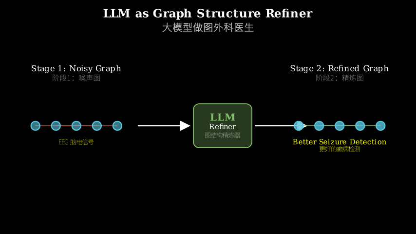
EEG-based seizure detection has converged on graph neural networks: treat electrode channels as nodes, construct edges based on signal correlations or learned patterns, then run GNN classifiers. The problem? EEG is inherently noisy—muscle artifacts, eye movements, electrical interference. Correlation-based methods create edges between channels that happen to wiggle together by accident. Learning-based methods overfit to spurious patterns. Both produce dense, messy graphs where real brain connectivity drowns in noise.

Prior work tried to fix this with better edge construction (attention mechanisms, adaptive thresholds, learnable adjacency matrices). But they’re still operating in feature space—no method has access to the semantic reasoning needed to ask “does this connection make neurological sense?”

Problem: Noisy EEG → Dense graphs with spurious edges
                              |
                              v
Assumption: LLMs can reason about edge validity using
            domain knowledge + statistical features
                              |
                              v
Method: Two-stage pipeline
        1. Transformer builds initial graph with edge probabilities
        2. LLM refines by validating each edge
                              |
                              v
Evidence: +3.8% accuracy on TUSZ, sparser graphs, 
          edges align with known brain connectivity
                              |
                              v
Conclusion: LLM reasoning > pure statistical learning
            for graph structure in noisy domains

The Increment

One sentence: Before—graph construction was a pure learning problem solved with neural architectures; after—it’s a two-stage process where learned structures get validated by LLM reasoning about domain semantics.

Core Mechanism

The method splits graph construction into generation and refinement. First stage: a Transformer encoder processes EEG time series from all channels, producing node embeddings. An MLP takes pairs of embeddings and outputs edge probability scores. Apply a threshold—edges above it survive to form the initial graph.

Second stage: the LLM receives each candidate edge as a structured prompt. The prompt contains: (1) textual features—channel names, brain regions, known functional roles; (2) statistical features—correlation coefficient, mutual information, edge probability from stage one. The LLM outputs a binary decision: keep or remove. Surviving edges form the final graph, which feeds into a standard GNN classifier for seizure detection.

EEG signals (channels × time)
         |
         v
   [Transformer Encoder]
         |
         v
   Node embeddings
         |
         v
   [MLP Edge Predictor] ---> Edge probabilities
         |                          |
         v                          |
   Threshold filter                |
         |                          |
         v                          |
   Candidate graph                 |
         |                          |
         +----------+               |
                    |               |
                    v               v
              [LLM Refiner]  <-- Textual + Statistical features
                    |
                    v
              Final graph
                    |
                    v
              [GNN Classifier] ---> Seizure / No seizure

Think of it like hiring a contractor to renovate a house. The Transformer is the demolition crew—it tears down walls (builds initial structure) based on blueprints (learned patterns). But demolition crews sometimes remove load-bearing walls or leave up walls that should go. The LLM is the structural engineer who walks through afterward with the building code (domain knowledge) and inspection tools (statistical features). For each wall, the engineer asks: “Does this make structural sense? Does it match the code? Do the measurements check out?” Walls that fail inspection get removed. The final structure is both data-driven (crew’s work) and semantically valid (engineer’s approval).

Key Concepts

• Graph edge refinement as reasoning task: Traditional graph learning treats edge existence as a continuous optimization problem—adjust weights via gradient descent until validation loss stops improving. This paper reframes it as a discrete reasoning problem: given evidence about a potential connection, should it exist? The shift matters because reasoning can incorporate non-differentiable knowledge (neuroanatomy, clinical guidelines) that gradient-based methods can’t access. The LLM doesn’t learn edge patterns from scratch; it validates them against a knowledge base acquired during pretraining. Concrete example: if the initial graph connects a frontal lobe channel to an occipital channel with high correlation (maybe both picked up the same electrical artifact), the LLM can reject it because those regions don’t typically show direct functional connectivity during seizures.

• Two-stage generation-refinement pipeline: Why not just use the LLM to build the entire graph from scratch? Cost and context limits. An EEG graph with 20 channels has 190 possible edges. Asking an LLM to reason about all 190 in one shot requires a massive prompt and burns tokens. The Transformer stage acts as a cheap filter—it uses learned patterns to propose a smaller candidate set (say, 50 edges). The LLM only reasons about these 50, making the approach tractable. The division of labor mirrors how humans work: quick heuristics narrow the search space, then careful reasoning validates the finalists.

Framework Shift

Before (mainstream approach):        After (this paper):

EEG signals                          EEG signals
     |                                    |
     v                                    v
[End-to-end GNN]                    [Transformer] 
     |                                    |
     | (learns adjacency                 v
     |  via backprop)              Candidate graph
     |                                    |
     v                                    v
Classification                      [LLM validates edges]
                                         |
                                         v
                                    Refined graph
                                         |
                                         v
                                    [GNN Classifier]
                                         |
                                         v
                                    Classification

Single-stage optimization           Two-stage: learn + reason
Implicit structure learning         Explicit structure validation

From monolithic neural optimization to hybrid neural-symbolic pipeline, the core shift is making graph structure an explicit reasoning target rather than an implicit learned artifact.

Expert Assessment

Problem choice: Real gap. EEG noise is a well-documented problem, and existing graph construction methods do produce messy adjacency matrices—you can verify this by visualizing learned graphs from prior work. The authors didn’t manufacture the problem. However, the gap sits in an incremental zone: improving graph quality for a specific application rather than rethinking seizure detection fundamentally.

Method maturity: Clever use of LLM capabilities, but the execution feels undercooked. The paper doesn’t explain how they engineered the LLM prompts—what exact format, how much context, whether they tried chain-of-thought or other prompting strategies. The Transformer+MLP stage is standard; the novelty is entirely in the LLM refinement, yet that component gets the least technical detail. Also, no ablation on whether a smaller, fine-tuned model could replace the LLM at lower cost.

Experimental integrity: Baselines are fair (correlation-based, attention-based, end-to-end learnable graphs). Numbers look reasonable—3.8% accuracy gain is meaningful in medical AI. But red flag: they only test on one dataset (TUSZ). EEG characteristics vary across hospitals, equipment, patient populations. Single-dataset results in medical AI are fragile. Also, no analysis of failure cases—when does the LLM make wrong refinement decisions?

Writing quality: The abstract and intro are clear. The method section is where it falls apart—Figure 2 (presumably the pipeline diagram) does heavy lifting, but the text doesn’t walk through a concrete example. The results section reports numbers but doesn’t show qualitative examples of refined graphs vs. initial graphs. Rewriting Section 3.2 (LLM refinement details) with explicit prompt templates and decision examples would elevate the paper significantly.

Verdict: weak accept — Interesting idea with promising results, but needs another revision to flesh out the LLM component and validate generalization across datasets.

Takeaways

Steal the two-stage pattern: When you have a noisy structured prediction problem (graphs, parse trees, knowledge bases), don’t force a single model to do everything. Use a fast learned model to generate candidates, then use a reasoning system (LLM, rule engine, constraint solver) to validate. The learned model handles scale; the reasoning system handles correctness.

LLMs as structure validators: If your domain has explicit knowledge (medical guidelines, physical laws, design principles) that’s hard to encode as differentiable losses, try using an LLM as a post-hoc filter. Frame each structural decision (edge existence, component placement, rule applicability) as a reasoning prompt with both learned features and domain context.

Prompt engineering matters more than the paper admits: The authors gloss over how they designed the LLM prompts, but that’s probably where most of the tuning effort went. If you replicate this approach, expect to spend time iterating on prompt format, feature selection, and output parsing. The paper’s results depend on getting that right, but they don’t share the recipe.