HyCNNs: Exponentially More Efficient Convex Neural Networks

Paper: 2604.26942 Authors: Shayan Hundrieser, Insung Kong, Johannes Schmidt-Hieber Categories: cs.LG, math.ST, q-bio.GN, stat.ME, stat.ML

The Gap

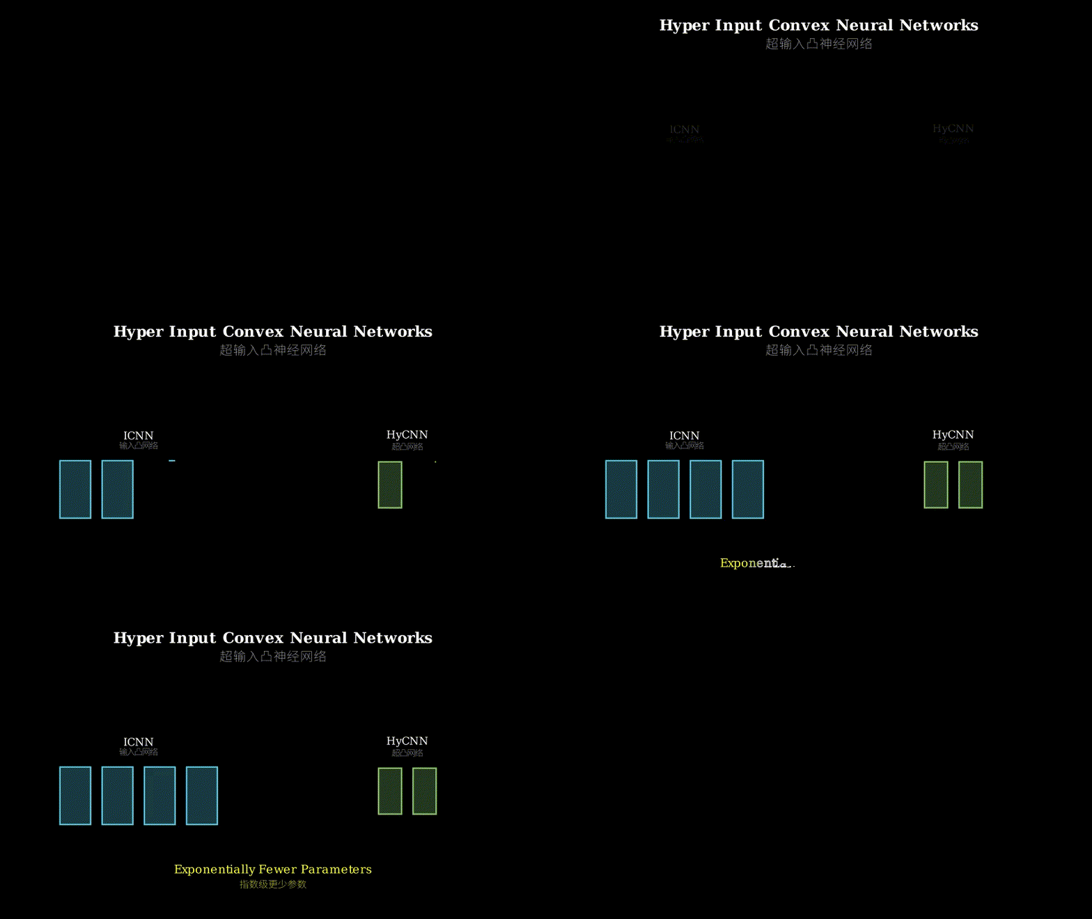
Input Convex Neural Networks (ICNNs) can learn functions that are guaranteed to be convex in their inputs — a property crucial for optimization, economics, and optimal transport. But ICNNs have a dirty secret: they scale terribly. To maintain convexity, they impose strict architectural constraints (non-negative weights, specific activation patterns) that cripple their expressiveness. The result? You need massive networks to approximate even simple convex functions like quadratics.

This matters because optimal transport — mapping one probability distribution to another — requires learning convex potential functions. Current ICNN-based methods either use enormous networks or settle for poor approximations. The field has been stuck choosing between theoretical guarantees (convexity) and practical efficiency (small networks).

Problem: Need convex functions for optimal transport
    |
    v
Constraint: ICNNs maintain convexity but need huge networks
    |
    v
Method: HyCNNs = Maxout structure + ICNN convexity rules
    |
    v
Evidence: Exponentially fewer params for quadratics, better transport maps
    |
    v
Conclusion: Can have both convexity guarantees AND efficiency

The Increment

One sentence: Before, you chose between convex guarantees with bloated networks (ICNNs) or efficient networks without guarantees (MLPs); now you get both through hierarchical max-pooling structure.

Core Mechanism

HyCNNs replace the standard ICNN layer structure with a hierarchical branching design. Each layer splits into multiple parallel branches, each computing a different affine transformation of the input. These branches then merge through a max operation — taking the pointwise maximum across all branches. This max-pooling happens at every layer, creating a tree-like structure where information flows through multiple paths before being combined.

The key insight: the max of convex functions is convex. So if you ensure each branch maintains convexity (using ICNN’s non-negative weight constraints), the entire network stays convex no matter how many branches you add. More branches mean more expressive power without sacrificing the convexity guarantee.

Input x
    |
    +----+----+----+
    |    |    |    |
   [W1] [W2] [W3] [W4]  <- parallel branches (affine transforms)
    |    |    |    |
    +----+----+----+
         |
       [MAX]  <- pointwise maximum
         |
    activation
         |
    next layer (repeat structure)

Think of HyCNNs like a river delta in reverse. A single river (your input) splits into multiple channels (branches), each flowing through its own terrain (affine transformation). At the confluence point, instead of merging by mixing waters, you keep only the highest water level at each location (max operation). This creates a new river that flows into the next split. Because water levels can only stay flat or rise when you take maximums (convexity), and each channel only raises the level (non-negative weights), the final water surface is guaranteed to be bowl-shaped (convex). The more channels you add, the more precisely you can sculpt that bowl’s shape, but you never lose the bowl property.

Key Concepts

• Input Convexity: A function f(x) is convex in x if the line segment between any two points on its graph lies above the graph itself. Visually, it’s bowl-shaped with no local valleys. Why does this matter? Convex functions have a single global minimum, making optimization reliable — gradient descent won’t get stuck in local minima. In optimal transport, the Kantorovich potential must be convex for the theory to work. Standard neural networks can’t guarantee this property; they might look convex on training data but curve the wrong way elsewhere.

• Maxout Networks: Instead of applying one activation function, Maxout computes multiple linear transformations and takes their maximum. If you have max(2x+1, -x+3, x-1), you’re essentially letting the network choose which linear piece to use at each input point. This creates a piecewise linear function that can approximate any continuous function. The “max” operation is the key — it’s both simple (just comparison) and powerful (creates sharp decision boundaries). Maxout was originally designed for better gradient flow, but here it’s repurposed to maintain convexity.

• Parameter Efficiency: ICNNs need width exponential in depth to approximate quadratics because their constrained structure (non-negative weights, specific activations) limits how much each layer can “bend” the function. It’s like trying to draw a curve using only straight lines that must point upward — you need many tiny segments. HyCNNs break this by using multiple branches per layer. Each branch can point in a different direction, and the max operation selects the highest at each point. This lets you approximate complex convex shapes with logarithmic depth instead of exponential width — the same way binary search beats linear search.

Framework Shift

Before (ICNNs):                    After (HyCNNs):

Input                              Input
  |                                  |
  v                                  +--+--+--+
[Layer] <- constrained             [B][B][B]  <- branches
  |         weights                  |  |  |
  v                                  +--+--+
[Layer]                               [MAX]
  |                                     |
  v                                     v
[Layer]                              [Layer]
  |                                  (repeat)
Output                              Output

Wide, shallow                      Narrow, deep
Many neurons per layer             Many branches per layer

From width-based expressiveness to depth-based expressiveness, the core shift is replacing neuron count with branching factor.

Expert Assessment

Problem choice: Real gap. Optimal transport is having a moment (single-cell biology, generative models, fair ML), and current neural methods genuinely struggle with high dimensions. The ICNN parameter explosion isn’t manufactured — it’s a known bottleneck in neural OT literature.

Method maturity: Clever insight, not brute force. The Maxout connection is elegant — both structures were known, but combining them to get convexity + efficiency is non-obvious. The exponential separation result (Theorem 3.1) is the paper’s backbone, showing this isn’t just empirical tinkering. However, the proof technique (approximating quadratics) is somewhat narrow; broader function classes would strengthen the claim.

Experimental integrity: Baselines are fair and comprehensive. They compare against ICNNs, standard MLPs, and existing neural OT methods across synthetic and real data. The single-cell RNA experiments are particularly strong — this is where practitioners actually use these methods. One concern: the paper doesn’t deeply investigate failure modes. When do HyCNNs struggle? The experiments show wins but don’t probe boundaries.

Writing quality: Section 3 (theory) is dense and could use more intuition before diving into proofs. The connection between Maxout and convexity preservation deserves a standalone subsection with visual examples. Section 5 (experiments) is well-structured but buries some important details (hyperparameter choices, training stability) in the appendix. Rewriting Section 3.1 to lead with geometric intuition would elevate the whole paper.

Verdict: strong accept — Solves a real problem with theoretical backing and strong empirical validation across multiple domains.

Takeaways

Architectural pattern: When you need a function property (convexity, monotonicity, Lipschitz bounds), look for operations that preserve that property under composition. Max preserves convexity; min preserves concavity; averaging preserves both. This “property-preserving composition” principle transfers beyond convexity — you can build networks with other guarantees using the same template.

Efficiency trick: When constrained architectures force you to go wide, try going deep with branching instead. The branching factor becomes your new expressiveness knob. This applies beyond neural nets — decision trees, ensemble methods, and even algorithm design use this width-to-depth trade.

Experimental design: The paper’s progression from synthetic (controlled) to semi-synthetic (realistic structure, known ground truth) to real (messy but meaningful) is a template worth stealing. Each level validates a different aspect: correctness, scalability, practical utility.

Red flag to watch: The paper doesn’t discuss training stability or convergence guarantees. HyCNNs have more hyperparameters (branch count per layer, depth) than ICNNs. If you’re adapting this, budget time for architecture search — the optimal branching structure likely depends on your problem’s geometry.