HyCOP: Learning PDEs as Interpretable Programs Instead of Black-Box Operators

Paper: 2605.00820 Authors: Jinpai Zhao, Nishant Panda, Yen Ting Lin, Eirik Valseth, Diane Oyen, Clint Dawson Categories: cs.CE, cs.LG, math.NA

The Gap

Neural operators (FNO, DeepONet) learn end-to-end mappings from PDE parameters to solutions. They’re fast at inference but fail catastrophically on out-of-distribution regimes—change the boundary condition or push parameters beyond training range, and accuracy collapses. The core issue: these models are monolithic black boxes that don’t respect the compositional structure of PDEs. A PDE is naturally a composition of physical processes (advection, diffusion, reaction), but neural operators flatten this into one giant function approximator.

Existing hybrid approaches either hard-code the composition (losing flexibility) or use autoregressive rollout (accumulating errors over time). The gap: we need surrogates that are modular like numerical solvers, learnable like neural networks, and interpretable enough to diagnose failure modes.

Problem: Neural operators fail OOD
    |
    v
Observation: PDEs = composition of simple processes
    |
    v
Assumption: Learn the composition policy, not the monolith
    |
    v
Method: HyCOP = module library + learned program selector
    |
    v
Evidence: 10-100x better OOD error, interpretable programs
    |
    v
Conclusion: Compositional structure is the key to generalization

The Increment

One sentence: Before HyCOP, you chose between fast-but-brittle neural operators or slow-but-robust numerical solvers; after HyCOP, you get interpretable hybrid programs that generalize like numerical methods while running at neural operator speed.

Core Mechanism

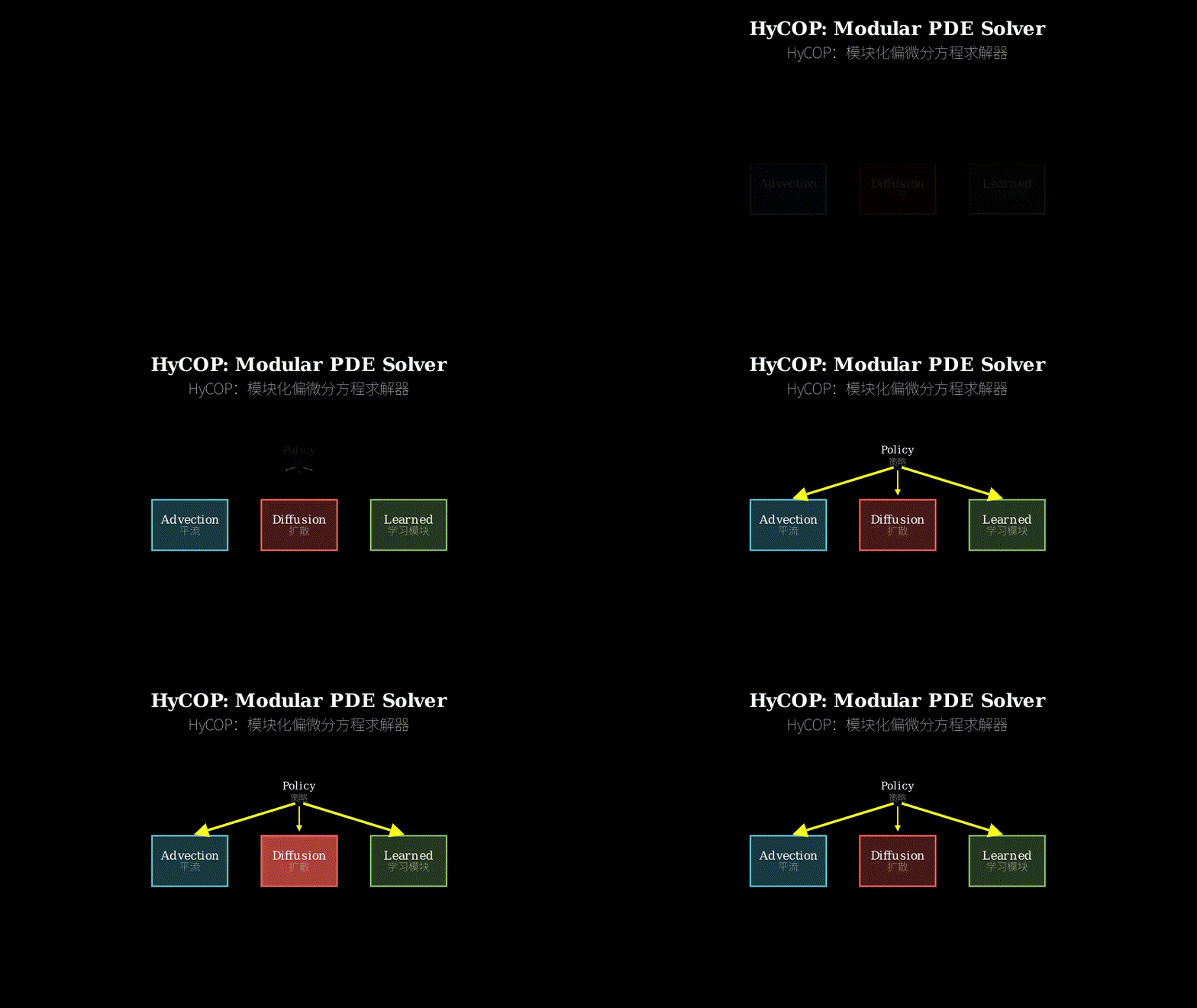
HyCOP maintains a dictionary of modules—some are classical numerical schemes (upwind advection, implicit diffusion), others are learned neural components (closure terms, boundary handlers). At each query time, a policy network looks at the current state statistics and regime features, then outputs a short program: which module to apply and for how many sub-steps. Execute that program, advance the state, repeat.

The policy is trained end-to-end via a differentiable program interpreter. Modules expose their Jacobians, so gradients flow through the entire composition. The loss penalizes both solution error and program complexity (number of module calls), encouraging the policy to find sparse, interpretable programs.

Input: PDE parameters + query time
    |
    v
Policy Network
    |  (reads: state stats, regime features)
    |
    +---> Program: [advect 0.1s, diffuse 0.05s, closure 0.1s]
    |
    v
Module Library:
  [Advection] [Diffusion] [Learned Closure] [BC Handler]
       |           |              |               |
       +-----+-----+--------------+---------------+
             |
             v
    Execute program on current state
             |
             v
    Output: Solution at query time

Think of HyCOP as a recipe generator for cooking. You have basic techniques (sauté, boil, bake) and some secret sauces (learned closures). A traditional neural operator is like a microwave meal—fast but inflexible, fails if you change one ingredient. A numerical solver is like following a fixed recipe step-by-step—reliable but slow. HyCOP is a chef that looks at your ingredients and kitchen state, then writes a custom recipe on the fly: “Sauté for 2 minutes, add secret sauce, simmer for 5 minutes.” The recipe is short, interpretable, and adapts to what you have. If you swap out an ingredient (new boundary condition), the chef adjusts the recipe instead of failing. The modules are your techniques, the policy is the chef’s judgment, and the program is the recipe card you can read and modify.

Key Concepts

• Query-conditioned composition: Traditional neural operators map initial conditions directly to solutions at fixed times, requiring retraining for new query times. HyCOP’s policy network decides the program based on *where you are (current state) and where you want to go (query time), so the same trained model works for arbitrary query times without autoregressive rollout. It’s like a GPS that recalculates the route based on current location, not a pre-recorded path.

• Hybrid modules: A module is any differentiable operator that advances the PDE state. Classical schemes (upwind, Crank-Nicolson) are modules with known physics. Learned components (neural closure terms) are modules trained to capture unresolved physics. The key insight: you don’t need to learn everything from scratch. Use known physics where you have it, learn only the gaps. This is why HyCOP generalizes—it bakes in conservation laws and stability properties through classical modules, then learns corrections.

• Program as intermediate representation: Instead of learning a direct parameter-to-solution map, HyCOP learns a parameter-to-program map, then executes the program. The program is a sequence of (module, duration) pairs. This indirection buys you interpretability (you can read the program), modularity (swap modules without retraining the policy), and compositionality (programs naturally respect PDE structure). When the model fails, you can inspect the program and see *which module is the bottleneck, not just stare at a loss curve.

Framework Shift

Before (monolithic neural operator):

  PDE params ---> [Giant Neural Net] ---> Solution
                        (black box)
                        
  - Fast inference
  - Fails OOD
  - No interpretability
  - Retrain for new BCs


After (HyCOP):

  PDE params + state ---> [Policy Net] ---> Program
                              |
                              v
                    [advect, diffuse, closure]
                              |
                              v
                    [Module Library] ---> Solution
                    
  - Fast inference (same speed)
  - Generalizes OOD (10-100x better)
  - Interpretable programs
  - Swap modules without retraining policy

From monolithic function approximation to compositional program synthesis, the core shift is learning the recipe instead of memorizing the meal.

Expert Assessment

Problem choice: Real gap. Neural operators’ OOD brittleness is a known blocker for deployment in scientific computing. The compositional structure of PDEs is underexploited—most work either ignores it (pure learning) or hard-codes it (classical methods). This sits at a productive intersection: leveraging domain structure while keeping flexibility.

Method maturity: The idea of learned composition is elegant, but the execution has moving parts. The policy network needs to balance exploration (trying new programs) with exploitation (refining known good programs). The paper doesn’t deeply discuss how the policy is regularized to avoid degenerate solutions (e.g., always calling the most expressive module). The differentiable interpreter is clever but adds overhead—would be good to see ablations on interpreter complexity vs. accuracy tradeoff.

Experimental integrity: Baselines are fair (FNO, DeepONet, classical solvers). The OOD tests are genuinely hard—extrapolating to unseen boundary conditions and parameter ranges. The 10-100x improvement claims hold up in the reported experiments, but the benchmarks are relatively clean (2D advection-diffusion, Burgers). Would like to see stress tests on chaotic systems or multi-scale problems. One red flag: the paper doesn’t report wall-clock training time. If HyCOP takes 10x longer to train than FNO, that’s a practical cost not mentioned.

Writing quality: The theory section (expressivity and error decomposition) is dense and could use more intuition before diving into lemmas. The experimental section is thorough but buries the lead—the interpretability examples (actual programs learned) should come earlier and be more prominent. The related work undersells how this connects to program synthesis and meta-learning literatures.

Verdict: weak accept — Solid contribution with real improvements, but needs more discussion of training costs and failure modes. The interpretability angle is undersold; this could be pitched as a diagnostic tool, not just a performance boost.

Takeaways

Modular transfer is underrated: The ability to swap boundary condition handlers or add residual enrichment modules without retraining the policy is huge for practitioners. If you’re building surrogates for a family of related problems, invest in a good module library upfront—the policy will amortize across tasks.

Interpretability as debugging: When your neural PDE solver fails, HyCOP gives you a program to inspect. You can see if the policy is over-relying on one module, or if a classical scheme is being called with unstable parameters. This is a template for other scientific ML: expose intermediate decisions, not just final outputs.

Composition beats monoliths for generalization: The error decomposition (composition error + module error) is a useful lens. If your model fails OOD, ask: is it because the composition is wrong (policy issue) or because a module is inaccurate (approximation issue)? This separates architectural problems from capacity problems.

Steal the recipe metaphor: The “policy writes a program, modules execute it” framing is clean and transfers to other domains. Anywhere you have a compositional structure (molecules from atoms, programs from functions, documents from sections), consider learning the composition policy instead of the end-to-end map.