Paper: 2606.12407 Authors: Kian R. Weihrauch, Thomas A. Buckley, William Lotter, Arjun K. Manrai Categories: cs.CV
The Gap
Prior work evaluated general-purpose LLMs on whole-slide images (WSIs) by feeding small, high-magnification patches (e.g., 256×256 at 20×) independently and aggregating via majority voting. Across benchmarks, these models consistently scored far below specialized pathology systems, leading the community to believe that architectural changes or extensive domain fine-tuning were required for any serious WSI task.
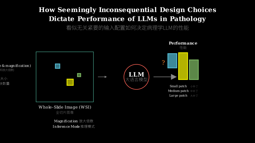
This paper steps back and asks: What if the input configuration – not the model – is the bottleneck? The authors systematically vary four factors (inference mode, patch size, magnification, patch count) in a full factorial design.
Problem: LLMs appear weak on WSI pathology (e.g., 15% on TCGA)
    |
    v
Assumption: gap is due to lack of domain-specific training
    |
    v
Method: factorial analysis of 4 input factors (inference_mode, patch_size, mag, count)
    |
    v
Evidence: optimal config gives GPT-5 39.5% on TCGA, 62.9% on GTEx
    |
    v
Conclusion: the assumed gap is largely an artifact of poor input choices
The Increment
One sentence: Before, the field thought LLMs needed special training for pathology; after this paper, we know that simply picking the right patch size, magnification, and inference strategy can close most of the gap.
Core Mechanism
The paper does not introduce a new model. Instead, it treats the input pipeline as a hyperparameter space and performs a grid search over four dimensions:
- Inference mode – majority vote (each patch gets an independent prediction) vs. joint inference (all patches fed together as a single prompt/sequence).
- Patch size – from 128×128 up to 1024×1024 pixels.
- Magnification – from 2.5× to 40× (simulated by downsampling the original 40× WSI).
- Patch count – the number of randomly sampled patches per WSI (e.g., 16, 32, 64, 128).
The data flow: a WSI → select N patches with given size and magnification → feed them to the LLM (either one-at-a-time with majority vote or all-at-once as a joint sequence) → obtain a classification.
[Data flow of factorial experiment]
+------------------+     +----------------------+     +-----------+
| WSI at 40x       | --> | Downsample to target  | --> | Sample N  |
| (whole slide)    |     | x0.5, x1, x2, ...    |     | patches   |
+------------------+     +----------------------+     +-----------+
                                                        |
                                                        v
                                     +----------------------------------+
                                     | Inference Mode                   |
                                     | [A] Majority vote: each patch    |
                                     |     -> LLM -> vote               |
                                     | [B] Joint: all patches           |
                                     |     -> LLM as single context     |
                                     +----------------------------------+
                                                        |
                                                        v
                                                   prediction
Structural metaphor: Think of the WSI as a *giant jigsaw puzzle painting that you want to classify (e.g., “is this a landscape or a portrait?”).
- Patch size = the size of the cardboard piece you look at. Tiny pieces (128×128) capture only a brushstroke; large pieces (1024×1024) reveal objects.
- Magnification = how close you hold the piece to your eyes. High magnification (40×) shows paint cracks but loses the big picture; low magnification (5×) shows the whole composition.
- Patch count = how many pieces you examine. Too few, you may miss the key feature; too many, you flood your brain (or the LLM’s context).
- Inference mode = your strategy for combining the pieces. *Majority vote means you look at each piece independently, shout “landscape!” or “portrait!”, and then count the shouts. Joint inference means you lay all the pieces on a table and look at them together, letting their spatial arrangement inform your decision.
The paper finds that for this task, it’s better to take a few large pieces at low magnification and look at them all together rather than many tiny close-up pieces voted independently. That’s the “balanced configuration” that jumps performance from 15% to 39%.
Key Concepts
- Factorial analysis: Instead of tweaking one knob at a time, the authors run experiments for all combinations of the four factors (a full factorial design). This reveals interactions – e.g., the best patch size depends on the magnification, and joint inference only helps when patches are large enough. Simple but often overlooked.
- Context window utilization: LLMs have a fixed context length (e.g., 128k tokens for GPT-5). Small, high-magnification patches waste tokens on redundant detail; large, low-magnification patches pack more semantic content per token, and joint inference allows the model to attend to relationships across patches.
- Domain transfer without tuning: The optimal configuration found on TCGA (cancer-type classification) transfers to GTEx (organ classification) and CPTAC (a fully held-out breast cancer cohort) without any parameter adjustment. This suggests the configuration benefit is a property of the input structure, not the label space.
Framework Shift
Here is the napkin sketch of the old practice vs. the new practice:
Before (mainstream approach):
+-----------+     +-------------+     +---------+
| Whole     | --> | tiny 256x256| --> | LLM     |
| Slide     |     | patches at 20x    | (per    |
| Image     |     | (e.g., 64 patches)| patch)  |
+-----------+     +-------------+     +---------+
                                          |
                                          v
                                     majority vote
                                          |
                                          v
                                      prediction

After (this paper's recommendation):
+-----------+     +-------------+     +---------+
| Whole     | --> | large 1024x  | --> | LLM     |
| Slide     |     | at 5x (e.g., |     | (joint) |
| Image     |     | 32 patches)  |     |         |
+-----------+     +-------------+     +---------+
                                          |
                                          v
                                     single prediction
From “many isolated close-ups → majority vote” to “few wide-angle views → joint reasoning,” the core shift is feeding the model more informative, less redundant patches while enabling it to combine information across them.
Expert Assessment
Problem choice: Real gap. Many prior LLM baselines in pathology were thrown together without thought to input design, and the community accepted the low scores as inherent. This paper surfaces a subtle but high-impact confound.
Method maturity: Clever but not deep. The experiment is a grid search – brute force by design. No new algorithm, no model change. The insight is in asking the right question, not in technical novelty.
Experimental integrity: Baselines are fair: they compare against the exact configs used in previous papers (small high-mag, majority vote). The factorial design is complete, and the hold-out cohort validates generalizability. Minor concern: “optimal” configs may be dataset-specific (though transfer results are encouraging). Also, the paper does not explore non-uniform patch sizes or adaptive sampling – possible improvements.
Writing quality: Clear and direct. The introduction could be shorter; the real meat is in the results tables. The “implications” section is the weakest – it ends too soon. A paragraph on practical guidelines for future WSI benchmarks would elevate the paper.
Verdict: Weak accept – Important empirical finding that every pathology-AI researcher should be aware of, but the method itself is simple factorial analysis.
Takeaways
- Always test input configuration before blaming the model. If you run an LLM baseline, try large patches (512–1024 at 5×–10×) and joint inference. This simple check can save months of “we need a specialized model” thinking.
- Majority voting is usually suboptimal for low-shot WSI classification. Joint inference allows the LLM to use its attention mechanism across patches, which matters more when you have few patches.
- Factorial analysis is underused in deep learning. When evaluating a pipeline, do a small grid over plausible input choices – the interaction effects can dwarf the effect of architecture changes.
- For transfer learning, the optimal input pipeline may be more robust than you expect. The config found on TCGA worked on GTEx and CPTAC without tuning; this suggests the pipeline shapes the input distribution in a dataset-agnostic way.
论文: 2606.12407 作者: Kian R. Weihrauch, Thomas A. Buckley, William Lotter, Arjun K. Manrai 分类: cs.CV
缺口
此前的工作评估通用LLM在全切片图像上的表现时,通常使用小的高放大倍数补丁(例如256×256像素,20倍放大),独立输入并通过多数投票聚合。 在多个基准上,这些模型的成绩始终远低于专业病理系统,导致学界普遍认为:为了任何严肃的WSI任务,都需要修改架构或进行大量领域微调。
本文退一步问:如果瓶颈在于输入配置,而非模型本身呢? 作者系统地对四个因素(推理模式、补丁大小、放大倍数、补丁数量)进行了全析因设计。
问题:LLM在病理WSI上表现差(例如TCGA上15%)
    |
    v
假设:差距源于缺乏领域专用训练
    |
    v
方法:对4个输入因素(推理模式、补丁大小、放大倍数、补丁数量)进行析因分析
    |
    v
证据:最优配置使GPT-5在TCGA达到39.5%,在GTEx达到62.9%
    |
    v
结论:假设的差距很大程度上是输入选择不当造成的假象
增量
一句话: 在这篇论文之前,学界认为LLM需要特殊训练才能胜任病理学任务;在这篇论文之后,我们知道只需选择合适的补丁大小、放大倍数和推理策略,就能弥合大部分差距。
核心机制
本文没有提出新模型。 相反,它将输入管线视为一个超参数空间,对四个维度进行全面网格搜索:
- 推理模式 – 多数投票(每个补丁独立预测) vs. 联合推理(所有补丁作为一个提示/序列输入)。
- 补丁大小 – 从128×128到1024×1024像素。
- 放大倍数 – 从2.5倍到40倍(通过对原始40倍WSI降采样模拟)。
- 补丁数量 – 每张WSI随机采样的补丁数(例如16、32、64、128)。
数据流:一张WSI → 选择N个给定大小和放大倍数的补丁 → 输入LLM(逐个输入并多数投票,或一次性作为联合序列) → 获得分类。
[析因实验的数据流]
+------------------+     +----------------------+     +-----------+
| 40倍WSI          | --> | 降采样到目标倍数     | --> | 采样N个   |
| (全切片)         |     | (0.5x, 1x, 2x, ...) |     | 补丁     |
+------------------+     +----------------------+     +-----------+
                                                        |
                                                        v
                                     +----------------------------------+
                                     | 推理模式                        |
                                     | [A] 多数投票:每个补丁          |
                                     |     -> LLM -> 投票              |
                                     | [B] 联合推理:所有补丁          |
                                     |     -> 作为单一上下文输入LLM    |
                                     +----------------------------------+
                                                        |
                                                        v
                                                   预测结果
结构隐喻: 把WSI看作一幅巨大的拼图画,你想要分类(例如“这是风景画还是肖像画?”)。
- 补丁大小 = 你看的拼图片的大小。小片(128×128)只能看到一笔一画;大片(1024×1024)能看见物体。
- 放大倍数 = 你把拼图片举到多近的眼前看。高倍(40×)能看到颜料裂纹,但失去整体构图;低倍(5×)能看到整个画面。
- 补丁数量 = 你检查多少块拼图片。太少可能漏掉关键特征;太多会淹没你的大脑(或LLM的上下文)。
- 推理模式 = 你组合拼图片的策略。**多数投票*是独立看每一块,喊“风景!”或“肖像!”,然后数票数。联合推理是把所有拼图片摆在一张桌子上一起看,让它们的空间布局帮助你决策。
本文发现,对于该任务,更好的做法是拿几块大的、低放大倍数的拼图片,然后一起看,而不是拿很多小的、高倍的拼图片独立投票。这就是使性能从15%跃升至39%的“平衡配置”。
关键概念
- 析因分析: 不是一次调一个旋钮,而是对所有四种因素的组合进行全面实验(全析因设计)。这能揭示交互作用——例如,最佳补丁大小依赖于放大倍数,且联合推理只在补丁足够大时才有效。方法简单,但常被忽视。
- 上下文窗口利用: LLM有固定的上下文长度(例如GPT-5的128k token)。小的高倍补丁在冗余细节上浪费token;大的低倍补丁每个token携带更多语义内容,而联合推理使模型能关注补丁间的关联。
- 无需调参的领域迁移: 在TCGA(癌症类型分类)上找到的最优配置无需任何参数调整即可迁移到GTEx(器官分类)和CPTAC(完全保留的乳腺癌队列)。这表明配置的好处来源于输入结构本身,而非标签空间。
框架转变
以下是旧实践与新实践的餐巾纸速写:
之前(主流方法):
+-----------+     +-------------+     +---------+
| 全切片    | --> | 小补丁256x256-->| LLM     |
| 图像      |     | 20倍放大      | (逐补丁)|
|           |     | (例如64个)    |         |
+-----------+     +-------------+     +---------+
                                          |
                                          v
                                     多数投票
                                          |
                                          v
                                     分类结果

之后(本文推荐):
+-----------+     +-------------+     +---------+
| 全切片    | --> | 大补丁1024x -->| LLM     |
| 图像      |     | 5倍放大       | (联合推理)|
|           |     | (例如32个)    |         |
+-----------+     +-------------+     +---------+
                                          |
                                          v
                                     单一预测
从“大量孤立的特写 → 多数投票”到“少量宽景视角 → 联合推理”,核心转变是向模型提供信息更丰富、冗余更少的补丁,同时使其能够跨补丁组合信息。
专家评审
选题眼光: 真缺口。此前很多病理学LLM基线在输入设计上非常随意,学界将低分视为模型本身的问题。本文揭示了一个微妙但影响巨大的混淆因素。
方法成熟度: 巧劲但不深。实验本质上是网格搜索——设计上是蛮力。没有新算法,没有模型改动。洞见在于提出了正确的问题,而非技术新颖性。
实验诚意: 基线公平:比较了此前论文使用的精确配置(小补丁、高放大、多数投票)。析因设计完整,保留队列验证了泛化性。细微顾虑:“最优”配置可能依赖数据集(虽然迁移结果令人鼓舞)。此外,本文未探索非均匀补丁大小或自适应采样——未来可能改进。
写作功力: 清晰直接。引言可以更短;真正的干货在结果表格中。“启示”部分最弱——结束得太早。如果有一段关于未来WSI基准实践指南的讨论,整篇论文会提升一个档次。
判决: 弱接收 – 重要的实证发现,每位病理AI研究者都应知晓,但方法本身只是简单的析因分析。
要点总结
- 在归咎模型之前,先测试输入配置。 如果你运行LLM基线,尝试大补丁(512–1024像素,5–10倍放大)和联合推理。这一简单检查可以节省数月“我们需要专门的模型”的思考时间。
- 对于低样本WSI分类,多数投票通常次优。 联合推理让LLM能够利用注意力机制跨补丁交互,当补丁数量较少时尤为重要。
- 析因分析在深度学习中未被充分使用。 评估管线时,应对合理的输入选择做一个小网格搜索——交互效应可能比架构变化的影响更大。
- 迁移学习中,最佳输入管线可能比你想象的更鲁棒。 在TCGA上找到的配置无需调参即可在GTEx和CPTAC上工作;这表明管线以一种与数据集无关的方式塑造了输入分布。