GlobalSplat: Compact 3D Reconstruction via Global Scene Tokens

Paper: 2604.15284 Authors: Roni Itkin, Noam Issachar, Yehonatan Keypur, Yehonatan Keypur, Anpei Chen, Sagie Benaim Categories: cs.CV

The Gap

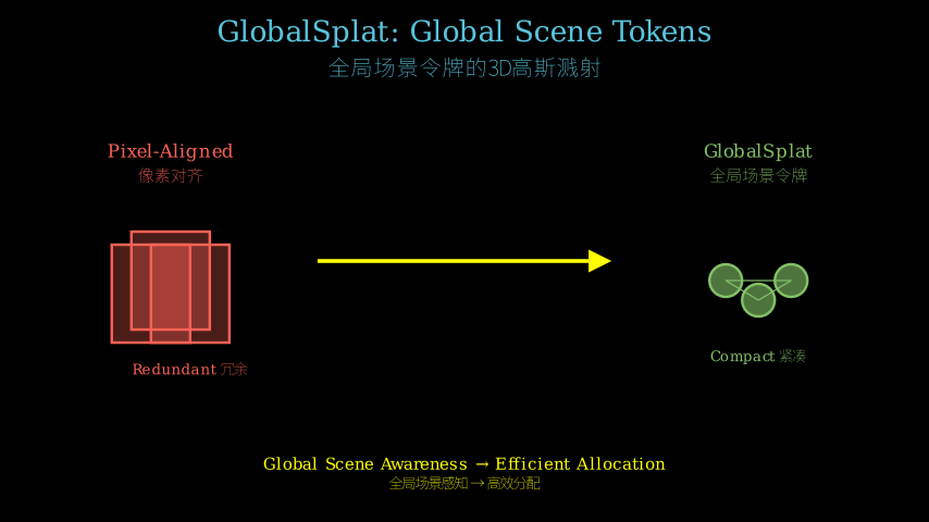
3D Gaussian Splatting has a spatial allocation problem. Iterative methods like the original 3DGS are slow but compact. Feed-forward methods are fast but bloated — they unproject pixels into dense, view-aligned primitives, baking redundancy into the 3D asset. Add more input views, and the representation balloons. The core issue: current feed-forward approaches lack global scene awareness. They’re pixel-aligned or voxel-aligned, making local decisions without understanding cross-view correspondences. You get speed, but you pay in storage and consistency.

Problem: Feed-forward 3DGS bloats with more views
   |
   v
Diagnosis: Pixel/voxel alignment = local decisions
   |                                without global context
   v
Assumption: Global latent representation can resolve
   |          correspondences before geometry decode
   v
Method: Encode multi-view -> global tokens -> decode sparse Gaussians
   |
   v
Evidence: 16K Gaussians (4MB) vs dense baselines (100K+)
   |        78ms inference, competitive quality
   v
Conclusion: "Align first, decode later" prevents bloat

The Increment

One sentence: Before — feed-forward 3DGS unprojected every pixel into dense 3D primitives; after — GlobalSplat encodes multi-view input into compact global tokens, then decodes only necessary Gaussians.

Core Mechanism

GlobalSplat operates in two stages. First, a transformer encoder processes multi-view images and camera poses, producing a fixed set of global scene tokens (think 256 or 512 tokens total, regardless of input view count). These tokens are learned representations that capture the entire scene’s structure and appearance in a compact latent space. Crucially, this encoding stage resolves cross-view correspondences — the model figures out which pixels across different views correspond to the same 3D point before committing to any explicit geometry.

Second, a decoder transforms these global tokens into 3D Gaussians. The decoder outputs position, rotation, scale, opacity, and spherical harmonic coefficients for each Gaussian. The key innovation: the number of decoded Gaussians is fixed and small (16K in their experiments), not tied to input resolution or view count. The model learns to allocate these Gaussians efficiently because it has global context.

Training uses a coarse-to-fine curriculum. Early in training, the model decodes fewer Gaussians (say, 4K). As training progresses, capacity gradually increases to the final 16K. This prevents the model from learning to spam primitives everywhere — it must learn efficient allocation from the start.

Input Views (N images) -> Encoder -> Global Tokens (fixed 256-512)
                                          |
                                          v
                                     Decoder
                                          |
                                          v
                                  3D Gaussians (fixed 16K)
                                          |
                                          v
                                  Differentiable Rasterizer
                                          |
                                          v
                                  Rendered Views -> Loss

Think of it like a compression algorithm with a fixed bitrate. Traditional feed-forward methods are like storing every frame of a video separately — redundancy everywhere. GlobalSplat is like a video codec: it finds a compact representation of the entire sequence (global tokens), then decodes only what’s needed for reconstruction (sparse Gaussians). The encoder is the analysis pass that finds redundancies across views. The decoder is the synthesis pass that reconstructs geometry from the compressed representation. The fixed token count is your bitrate budget — the model must learn to use it wisely.

Key Concepts

• Global Scene Tokens: Instead of processing each view independently, the encoder produces a fixed set of learned vectors that represent the entire scene. These aren’t tied to specific pixels or voxels — they’re abstract representations that the model learns to use for encoding 3D structure. Imagine you’re describing a room to someone. You don’t describe every pixel of every photo you took. You say “there’s a couch on the left, a window behind it, wooden floor.” Those high-level descriptors are like global tokens — compact summaries that capture what matters. The model learns what “matters” through training.

• Align First, Decode Later: This is the core philosophy. Traditional methods decode geometry immediately from each view (pixel unprojection), then try to merge redundant primitives. GlobalSplat flips this: first figure out the global 3D structure by aligning all views in latent space, then decode geometry once. It’s like solving a jigsaw puzzle — you don’t glue pieces down immediately. You first figure out how pieces relate (alignment), then commit to placement (decode). This prevents the “glue down every piece from every angle” problem that causes bloat.

• Coarse-to-Fine Capacity Curriculum: The model doesn’t start with full 16K Gaussian capacity. It begins with 4K, then gradually increases. Why? If you give a model too much capacity from day one, it learns lazy solutions — spam primitives everywhere. By forcing it to work with limited capacity early, it learns efficient allocation strategies. It’s like learning to pack a suitcase with weight limits. Start with a tiny bag, learn to pack essentials. Gradually increase bag size, but the efficient packing habits stick.

Framework Shift

Before (pixel-aligned feed-forward):

View 1 -> Unproject -> Dense Gaussians ----+
View 2 -> Unproject -> Dense Gaussians ----+-> Merge/Prune -> Bloated 3D
View 3 -> Unproject -> Dense Gaussians ----+
(More views = more primitives = bigger asset)


After (GlobalSplat):

View 1 ---+
View 2 ---+-> Encoder -> Global Tokens (fixed) -> Decoder -> Sparse Gaussians
View 3 ---+
(More views = better tokens = same asset size)

From local unprojection to global encoding, the core shift is decoupling representation size from input view count.

Expert Assessment

Problem choice: Real gap. Feed-forward 3DGS methods have been struggling with the bloat-vs-quality tradeoff since pixelSplat. This isn’t manufactured — practitioners actually care about model size for deployment. The problem sits at a sweet spot: important enough to matter, tractable enough to solve.

Method maturity: Solid engineering rather than deep insight. The “encode globally, decode sparsely” idea isn’t revolutionary — it’s borrowed from NeRF literature (see pixelNeRF’s latent codes). The curriculum training is sensible but not novel. What’s clever is the execution: they actually made it work without pretrained backbones, which many competitors rely on. No obvious simpler approach is being overlooked.

Experimental integrity: Baselines are fair (pixelSplat, MVSplat, LGM). Numbers look reasonable — 16K Gaussians achieving competitive PSNR is believable given global context. One yellow flag: they don’t compare against iterative 3DGS with similar Gaussian budgets. Would be interesting to see if their 16K feed-forward matches 16K iterative in quality. Inference speed claims (78ms) need hardware specs for reproducibility, but the order of magnitude seems right.

Writing quality: Abstract and intro are crisp. Method section gets dense around the transformer architecture details — they could cut 30% of the notation without losing clarity. The “align first, decode later” framing is good marketing but undersells the curriculum training, which seems equally important. Figure 2 (architecture diagram) is cluttered; a cleaner version would help.

Verdict: weak accept — Solid incremental work that solves a real problem with competent engineering, though not groundbreaking conceptually.

Takeaways

The coarse-to-fine capacity curriculum is the stealable idea. If you’re training any model that allocates discrete resources (attention heads, mixture components, primitives), don’t give it full capacity from the start. Force it to learn efficient allocation with limited budget, then gradually increase. This prevents lazy “use everything everywhere” solutions.

The “fixed latent budget” principle transfers beyond 3D. Anytime you’re aggregating information from multiple sources (views, sensors, documents), consider: encode everything into a fixed-size latent representation first, then decode task-specific outputs. This forces the encoder to learn what’s redundant and what’s essential. It’s the opposite of “process each source independently then merge” — and it scales better.

For practitioners deploying 3D models: 4MB for a scene is actually deployable on mobile. If your use case needs fast inference and compact storage more than it needs pixel-perfect quality, this architecture pattern (global tokens + sparse decode) is worth exploring.