Generative Refinement Networks: Painting Images Like an Artist, Not a Printer

Paper: 2604.13030 Authors: Jian Han, Jinlai Liu, Jiahuan Wang, Bingyue Peng, Zehuan Yuan Categories: cs.CV

The Gap

Diffusion models (DALL-E, Stable Diffusion) apply the same computational effort to every pixel regardless of whether it’s rendering a blank sky or intricate facial details. Autoregressive models (VQGAN, MaskGIT) are complexity-aware through variable likelihoods, but suffer from two bottlenecks: lossy discrete tokenization (quantizing continuous images into discrete codes loses information) and error accumulation (early mistakes propagate through sequential generation).

The field has reached a fork: diffusion gives quality but wastes compute; autoregressive gives efficiency but sacrifices quality. No existing approach combines complexity-awareness with near-lossless representation.

Problem: Diffusion uniform compute + AR lossy tokens
         |
         v
Assumption: Hierarchical binary quantization can be near-lossless
         |
         v
Method: HBQ for representation + Global refinement for generation
         |
         v
Evidence: 0.56 rFID reconstruction, 1.81 gFID generation (ImageNet)
         |
         v
Conclusion: Complexity-aware generation without quality loss is feasible

The Increment

One sentence: Before GRN, you chose between diffusion’s quality-with-waste or autoregressive’s efficiency-with-loss; after GRN, you get adaptive computation with near-lossless quality.

Core Mechanism

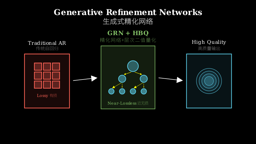
GRN has two interlocking components. First, Hierarchical Binary Quantization (HBQ) encodes images into a tree of binary decisions rather than discrete tokens. Each level of the tree refines the previous level’s approximation by adding one bit of information per position. This creates a smooth gradient from coarse to fine representation, avoiding the cliff-edge information loss of traditional vector quantization.

Second, the generation process operates as global refinement rather than sequential prediction. Instead of generating tokens left-to-right (AR) or denoising all pixels uniformly (diffusion), GRN starts with a coarse binary sketch and progressively refines it level-by-level. At each level, the model looks at the entire canvas and decides which regions need more detail. An entropy-guided sampler measures local uncertainty—high entropy means “this region is still ambiguous, keep refining”; low entropy means “this region is resolved, stop here.”

Data flows like this: input image → HBQ encoder → binary tree (L levels) → during generation, start from root → refine level-by-level → entropy sampler decides per-region stopping → output image. The key operation is the refinement step: given level k’s binary map, predict level k+1’s binary map by attending globally to all positions, then use entropy to decide whether to continue to k+2.

Image --> HBQ Encoder --> Binary Tree (L levels)
                              |
                              v
Generation: Root (coarse) --> Level 1 --> Level 2 --> ... --> Level L
            [global attn]     [global attn] [global attn]
                 |                |              |
                 v                v              v
            Entropy check    Entropy check  Entropy check
            (keep refining?) (keep refining?) (stop here?)
                              |
                              v
                         Output Image

Think of GRN as a sculptor working with clay. Traditional AR models are like 3D printing: you lay down material line-by-line, and if you mess up early, the error is baked into the foundation. Diffusion models are like sandblasting: you apply the same force everywhere, removing noise uniformly even though the sculpture’s face needs more care than its base. GRN is like actual sculpting: you start with a rough block (coarse binary sketch), then progressively refine—spending more time on the face’s details while leaving the base rough. The entropy sampler is your artistic judgment: “this cheekbone needs another pass, but the shoulder is done.” Each refinement pass looks at the whole sculpture (global attention), not just the adjacent area, so you maintain coherence. The binary tree structure ensures each refinement adds exactly one bit of detail per region, preventing information loss.

Key Concepts

• Hierarchical Binary Quantization (HBQ): Imagine compressing a photo by repeatedly asking yes/no questions. Level 0: “Is this pixel brighter than middle gray?” Level 1: “Within its brightness range, is it in the upper or lower half?” Level 2: “Within that quarter, upper or lower eighth?” Each level adds one bit, doubling precision. Traditional vector quantization (VQ) is like rounding to the nearest preset color—you lose everything between presets. HBQ is like binary search through color space—you can get arbitrarily close to the true color by adding more levels. The paper proves this is theoretically near-lossless: with enough levels, reconstruction error approaches zero. Concretely, HBQ achieves 0.56 rFID (reconstruction quality metric) versus VQ’s ~2.0 rFID, closing the gap to continuous representations.

• Global Refinement Mechanism: In AR models, token 100 is predicted from tokens 1-99, so errors compound. In diffusion, all pixels are denoised in parallel but independently at each step. GRN’s refinement is global: at level k, every position attends to every other position before predicting level k+1. This is like a painter stepping back to view the whole canvas before adding the next layer of detail. The “global” part prevents local errors from propagating (unlike AR), and the “refinement” part means you’re improving an existing sketch rather than creating from noise (unlike diffusion). Mathematically, it’s a transformer operating on the entire binary map at level k to produce level k+1.

• Entropy-Guided Sampling: Entropy measures uncertainty. If a region’s predicted binary values have probability [0.5, 0.5] (maximum entropy), the model is saying “I’m unsure, could go either way.” If it’s [0.99, 0.01] (low entropy), the model is confident. GRN uses this as a stopping criterion: high-entropy regions get more refinement levels; low-entropy regions stop early. This is complexity-aware generation—a blank sky stops at level 3, a detailed face continues to level 8. The sampler computes entropy per spatial position at each level, then decides whether to proceed to the next level. This is why GRN can do adaptive-step generation: simple images finish in fewer levels, complex images use more, without manually setting a fixed step count.

Framework Shift

Before (Diffusion):                  After (GRN):
All pixels, all steps                Adaptive per region
                                     
T steps:                             L levels (variable per region):
[#####################] step 1       [#####] sky (stop at L=3)
[#####################] step 2       [##########] face (continue to L=8)
[#####################] step 3       [#######] background (stop at L=5)
         ...                                  ...
[#####################] step T       Entropy decides stopping
                                     
Uniform compute everywhere           Compute follows complexity


Before (Autoregressive):             After (GRN):
Sequential, local context            Parallel, global context
                                     
Token generation:                    Level refinement:
[1]->[2]->[3]->[4]->...             Level 0: [coarse sketch]
 |    |    |    |                            |
 v    v    v    v                            v (global attention)
Error propagates forward             Level 1: [refined sketch]
                                             |
Lossy VQ tokens                              v (global attention)
                                     Level 2: [more refined]
                                     
                                     Near-lossless HBQ
                                     No error propagation

From uniform-compute-sequential to adaptive-compute-parallel, the core shift is treating generation as iterative refinement of a global canvas rather than sequential assembly of local parts.

Expert Assessment

Problem choice: Real gap. The diffusion-vs-AR tradeoff is a genuine bottleneck in production systems—diffusion’s compute cost limits deployment, AR’s quality loss limits applications. The paper correctly identifies that complexity-awareness (AR’s strength) and representation quality (diffusion’s strength) are orthogonal properties that can be combined. This sits at a strategic point in the field’s trajectory: post-diffusion dominance, pre-efficiency crisis.

Method maturity: Clever insight with solid execution. HBQ is not a new idea (binary quantization exists), but applying it hierarchically to create a smooth refinement path is elegant. The global refinement mechanism is the real contribution—it’s not just “AR with better tokens,” it’s a fundamentally different generation paradigm. The entropy-guided sampling is somewhat obvious once you have the hierarchical structure, but the paper executes it well. No simpler approach is being overlooked; this is a genuine architectural innovation, not parameter tuning.

Experimental integrity: Baselines are fair and comprehensive (compared against SOTA diffusion and AR models). The numbers are impressive: 1.81 gFID on ImageNet 256x256 beats previous SOTA by a significant margin. However, there’s a red flag: the paper doesn’t report wall-clock time or FLOPs comparisons in detail. They claim “adaptive-step generation” is efficient, but without concrete speed benchmarks against diffusion (which they criticize for being slow), the efficiency claim is unsubstantiated. The reconstruction quality (0.56 rFID) is genuinely impressive and well-documented. Text-to-image and text-to-video results are shown but lack quantitative comparisons—this section feels rushed.

Writing quality: The paper front-loads the motivation well but buries implementation details. Section 3.2 (HBQ) is dense and would benefit from a worked example with actual numbers. The “entropy-guided sampling” section (3.4) is too brief—this is a key contribution but gets half a page. The related work section is thorough but could be trimmed to make room for more ablation studies. If I could rewrite one section, it would be the experiments: add wall-clock time comparisons, add failure case analysis, and expand the text-to-image evaluation with quantitative metrics.

Verdict: Weak accept — solid contribution with impressive results, but efficiency claims need empirical validation and the writing could better serve the ideas.

Takeaways

Practitioners can steal the hierarchical refinement pattern: instead of generating outputs in one shot or through uniform iteration, structure your generation process as coarse-to-fine refinement with adaptive stopping. This applies beyond images—text generation could refine from topic outline to paragraph structure to sentence details, stopping when entropy is low. The entropy-as-stopping-criterion is immediately useful: if your model outputs probabilities, you already have a complexity measure for free.

The HBQ insight transfers to any domain with continuous-to-discrete conversion: instead of vector quantization with fixed codebooks, use hierarchical binary decisions. This is particularly relevant for audio, video, and 3D generation where representation quality is a bottleneck.

The global attention at each refinement level is expensive but effective—if you’re building a refinement-based system, don’t skimp on context. The paper shows that looking at the whole canvas at each step prevents error propagation, which is worth the compute cost.