Generative Drifting Unmasked: It's Score Matching with a Frequency Problem

Paper: 2603.09936 Authors: Erkan Turan, Maks Ovsjanikov Categories: cs.LG

The Gap

Generative Drifting recently achieved state-of-the-art one-step image generation using a kernel-based drift operator. The results were impressive, but the method was essentially a black box—it worked, but nobody knew why. Three critical questions remained unanswered: Does zero drift actually guarantee the distributions match? How do you pick the right kernel? And why does training collapse without the mysterious “stop-gradient” operator?

The prior landscape: Score-based diffusion models dominate generative modeling with solid theory (score matching, SDEs, denoising). Flow matching provides an alternative with straight trajectories. But drifting sat outside this theoretical ecosystem—a kernel trick that worked empirically but lacked the mathematical scaffolding to understand its behavior or improve it systematically.

Empirical Success (Drifting)
         |
         v
    [Black Box]  <--- Why does it work?
         |            Which kernel?
         v            Why stop-gradient?
    SOTA Results
         |
         v
    [Theory Gap] ---> This Paper
         |
         v
    Score Matching Connection
         |
         v
    Spectral Analysis + Gradient Flow
         |
         v
    Answers to All Three Questions

The Increment

One sentence: Before this paper, drifting was an empirical kernel trick; after, it’s a principled score-matching method with frequency-dependent convergence theory and a variational foundation.

Core Mechanism

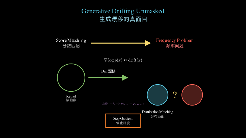
The drift operator takes samples from a source distribution and pushes them toward a target distribution using a kernel-weighted difference. The key insight: under a Gaussian kernel, this drift is mathematically identical to computing the score difference between smoothed versions of the two distributions. This connects drifting to the well-studied score-matching framework.

The method works by: (1) smoothing both distributions with a kernel, (2) computing their score functions (gradients of log-densities), (3) taking the difference, and (4) using this as the drift direction. The stop-gradient operator prevents the target distribution’s score from backpropagating gradients, which turns out to be essential for maintaining the gradient flow structure.

The spectral analysis reveals why kernel choice matters. By linearizing the McKean-Vlasov dynamics and analyzing in Fourier space, the authors show that different frequencies (fine vs coarse features) converge at different rates. Gaussian kernels suffer an exponential bottleneck for high frequencies—like trying to sculpt fine details with a very wide brush. Laplacian kernels handle high frequencies better, explaining their empirical superiority.

Source Samples (p)          Target Samples (q)
      |                            |
      v                            v
  [Kernel Smooth]            [Kernel Smooth]
      |                            |
      v                            v
  Smoothed p                 Smoothed q
      |                            |
      v                            v
  [Compute Score]            [Compute Score]
      |                            |
      |                            v
      |                    [Stop-Gradient] <-- Critical!
      |                            |
      +----------> [Difference] <--+
                        |
                        v
                  Drift Direction
                        |
                        v
                  Update Samples

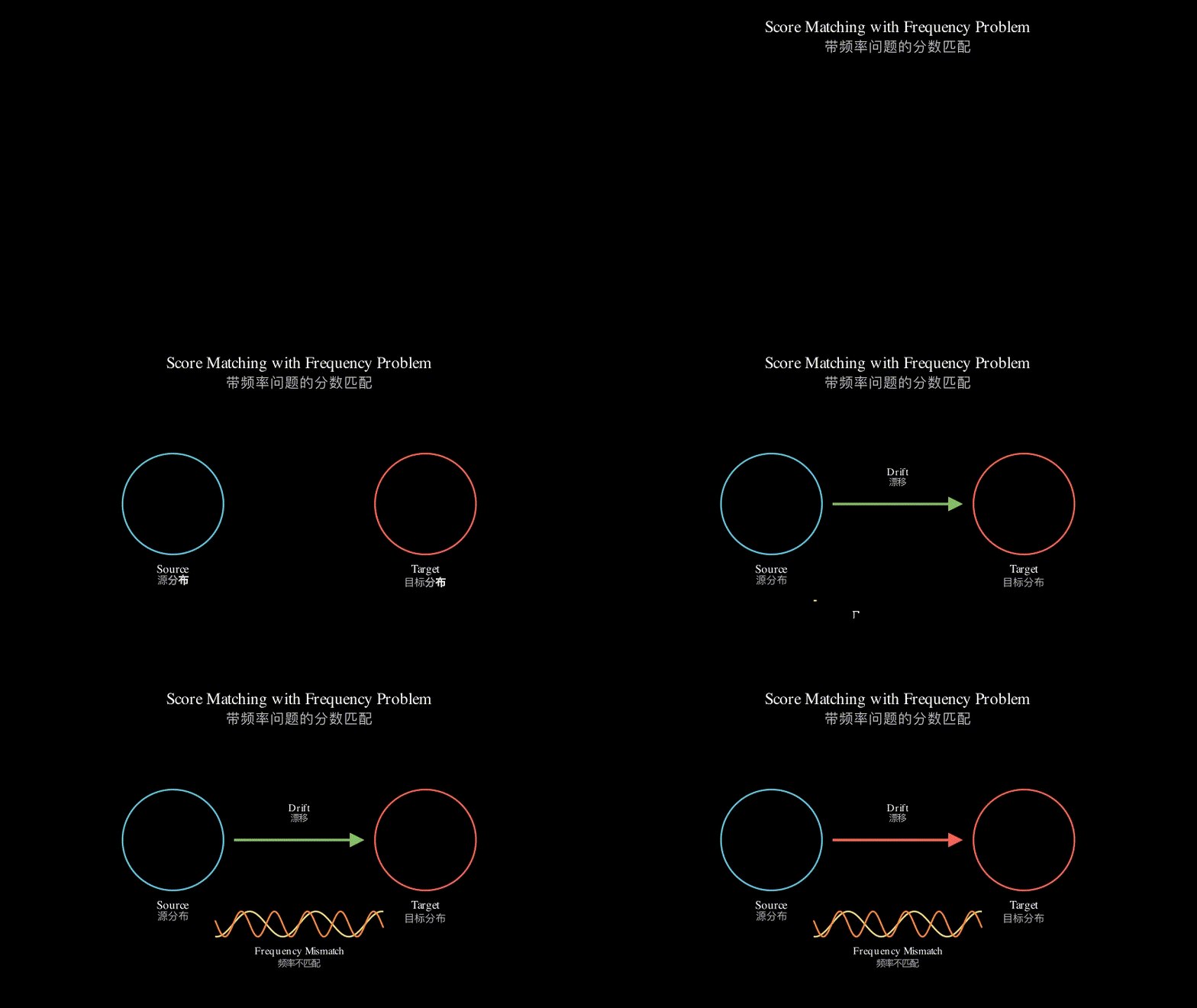
Think of it like audio equalization. You have a source sound (distribution) and want to match a target sound. The drift operator is like adjusting frequency bands—but here’s the catch: the Gaussian kernel is like having a very wide equalizer slider that affects many frequencies at once. When you try to adjust high frequencies (fine details), you inevitably mess with nearby frequencies too. This creates an exponential slowdown for high-frequency convergence—the “Landau damping” effect borrowed from plasma physics.

The Laplacian kernel is like having sharper, more independent frequency controls. Each frequency band can be adjusted without bleeding into others as much. The exponential bandwidth annealing schedule is like starting with wide sliders (fast broad adjustments) and gradually narrowing them (precise fine-tuning), reducing convergence time from exponential to logarithmic in the maximum frequency.

The stop-gradient operator is like freezing the target equalizer settings while you adjust the source. Without it, both would be moving simultaneously, creating feedback loops that destroy the gradient flow structure—like trying to match two moving targets instead of one fixed reference.

Key Concepts

• Score Matching: Imagine you have a probability distribution over images, but you don’t know its exact form—you only have samples. The “score” is the gradient of the log-probability: it points in the direction where probability density increases fastest. Score matching means learning this gradient field without ever computing the actual probabilities (which is intractable for high-dimensional data). In practice, you train a neural network to predict these gradients by matching them to the gradients of a known smoothed version of your data distribution. It’s like learning the terrain’s slope at every point without ever seeing the full topographic map.

• Drift Operator: In the context of moving probability distributions, drift is the velocity field that pushes samples from one distribution toward another. Think of it like a vector field in physics—at each point in space, there’s an arrow telling you which direction to move. For generative modeling, you start with noise (easy to sample) and the drift operator tells each noise sample how to evolve into a data sample. The kernel-based drift computes this by looking at the difference between source and target distributions, weighted by how “close” points are (determined by the kernel).

• Spectral/Fourier Analysis: Every signal or distribution can be decomposed into frequencies—low frequencies capture broad patterns, high frequencies capture fine details. In image generation, low frequencies are like the overall composition and lighting, while high frequencies are edges and textures. The spectral analysis here reveals that the drift operator converges at different speeds for different frequencies. Gaussian kernels create an exponential bottleneck: high frequencies take exponentially longer to converge. This is why generated images might get the overall structure right quickly but struggle with fine details—the math literally shows high frequencies are exponentially harder to match.

Framework Shift

Before (Empirical Drifting):        After (This Paper):

Source ---> [Kernel] ---> Target    Source ---> [Score] ---> Drift
  p            ???           q         p          Match         
                                                   |
[Black Box Operator]                    [Wasserstein Gradient Flow]
                                                   |
Works but why?                          Smoothed KL Divergence
                                                   |
                                        [Spectral Analysis]
                                                   |
                                        Frequency-dependent
                                        convergence rates

From mysterious kernel trick to principled gradient flow, the core shift is recognizing that drifting is score matching on smoothed distributions, enabling rigorous analysis of convergence behavior through spectral theory.

Expert Assessment

Problem choice: This is a real gap, not manufactured. When a method achieves SOTA results but lacks theory, that’s a genuine research opportunity. The three open questions are natural and important—practitioners need to know if their training objective is sound, how to choose hyperparameters, and why certain tricks are necessary. The timing is good: drifting is recent enough to be relevant but established enough to warrant theoretical investigation.

Method maturity: The connection to score matching is elegant—it’s the kind of insight that seems obvious in hindsight but required careful analysis to uncover. The spectral analysis borrowing from plasma physics (Landau damping) is sophisticated and non-obvious. However, the exponential bandwidth annealing feels somewhat incremental—it’s a natural next step once you understand the frequency bottleneck. The Wasserstein gradient flow formalization is solid but could have been developed more deeply.

Experimental integrity: The paper is primarily theoretical, which is appropriate given its goals. The spectral analysis is mathematically rigorous. The exponential annealing schedule shows clear improvements (exp to log convergence), though empirical validation on actual image generation tasks would strengthen the claims. The Sinkhorn divergence drift is mentioned as a demonstration but not thoroughly evaluated—this feels like a teaser for future work rather than a complete contribution.

Writing quality: The abstract is dense and assumes significant background. The connection to Landau damping is fascinating but might alienate readers unfamiliar with plasma physics—a more accessible analogy earlier would help. The paper jumps between spectral analysis, variational perspectives, and practical implications without always signposting the transitions clearly. The section on stop-gradient could be expanded—it’s treated somewhat tersely given its importance. Rewriting the introduction to build intuition before diving into technical details would make the paper more accessible.

Verdict: weak accept — Solid theoretical contribution that explains an empirically successful method, but lacks comprehensive empirical validation and could improve accessibility.

Takeaways

For practitioners: If you’re using drifting or similar kernel-based methods, this paper tells you to prefer Laplacian kernels over Gaussian for better high-frequency convergence. The exponential bandwidth annealing schedule (σ(t) = σ₀e^(-rt)) is immediately applicable—start with large bandwidth and decay exponentially during training for faster convergence.

For researchers: The spectral analysis framework is transferable. Whenever you have a distribution-matching method with a smoothing parameter, analyze it in Fourier space to understand frequency-dependent behavior. The connection between stop-gradient and JKO discretization provides a principled way to think about gradient flow discretizations—if your method should be a gradient flow, check whether your discretization preserves that structure.

For theorists: The paper demonstrates how to bridge empirical methods and established theory. When a new method works but lacks explanation, look for connections to existing frameworks (here, score matching). The variational perspective (Wasserstein gradient flow of smoothed KL) provides a template for deriving new drift operators from different divergences—the Sinkhorn example hints at this but isn’t fully explored.

The most concrete steal: if you’re training any generative model with a bandwidth/smoothing parameter, don’t keep it fixed—anneal it exponentially. The math shows this can turn exponential convergence into logarithmic.