Feeling the Curvature Blindfolded: Curvature-Aware Zeroth-Order Test-Time Adaptation

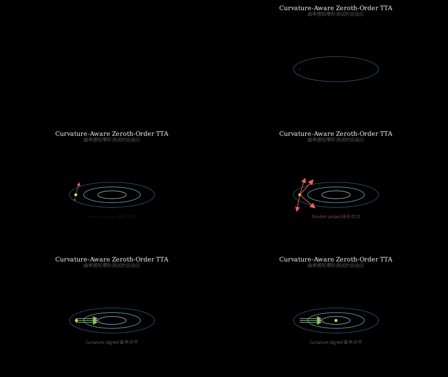
Paper: 2608.12279 Authors: Junming Zhang, Shuyu Yin, Peilin Liu, Rendong Ying, Fei Wen Categories: cs.CV

The Gap

Test-time adaptation is by now a crowded field, and almost all of it assumes backpropagation. TENT minimizes prediction entropy through the BatchNorm affine parameters; EATA adds sample filtering and a Fisher anchor; SAR swaps in sharpness-aware updates so it survives tiny or imbalanced batches; CoTTA and MEMO go further with augmentation-consistency and teacher-student machinery. Every one of them needs a backward pass, which means keeping the activation cache alive across the whole depth of the network. On a phone or an embedded NPU, that cache — not the weights — is what blows the memory budget. Many deployment stacks do not even ship a training runtime.

The BP-free branch is much thinner. FOA (forward-only adaptation) attacks the problem with CMA-ES over prompt tokens plus an activation-shifting trick, and MeZO showed in the LLM world that a two-forward-pass SPSA estimator can fine-tune at inference-level memory. Both inherit the curse of zeroth-order optimization: you are estimating a gradient from scalar loss differences along random directions, and the variance of that estimate grows with the number of parameters you are probing. In practice ZO-based adaptation is slower, noisier, and usually a couple of accuracy points behind its BP-based cousins — which is exactly why people keep paying for backprop.

The paper’s wedge is an empirical claim: during test-time adaptation, the loss Hessian over the adapted parameters is persistently low-rank. Only a handful of directions carry real curvature; the rest of the space is nearly flat. If that is true, isotropic probing is wasteful almost by construction — most of every random direction you sample lands in a subspace where the loss barely responds. So reshape the sampling distribution to match the curvature, and you get variance reduction for free.

[Problem] on-device TTA: BP requires activation cache + training runtime
     |
     v
[BP-free option] ZO / SPSA: forward passes only, inference-level memory
     |
     v
[Blocker] isotropic random probes: gradient-estimate variance scales
     |     with the probed dimension; ZO-TTA lags BP-TTA
     v
[Observation] during TTA the loss Hessian stays LOW-RANK and stable
     |         (a few directions hold nearly all the curvature)
     v
[Method] CAZO: sliding-average diagonal Hessian, harvested from the
     |   same two probes, defines an anisotropic sampling covariance
     v
[Evidence] cross-domain image benchmarks: beats prior TTA methods while
     |   holding memory near forward-only cost; ablations vs isotropic ZO
     v
[Conclusion] the bottleneck in ZO-TTA was probe *shape*, not probe *count*

The Increment

One sentence: Before, backprop-free test-time adaptation meant accepting isotropic random search and its accuracy tax; after, the two forward probes you were already paying for also tell you where the loss curves, and you spend your probing budget only there.

Core Mechanism

Start with the setup. The pretrained backbone is frozen — no gradients, no activation cache, no optimizer state for the bulk of the model. Only a small adapter (a low-dimensional set of trainable parameters inserted into the network) is optimized. This matters twice over: it is what keeps memory at inference level, and it shrinks the dimension that ZO variance depends on. Then, per test batch, an unsupervised objective in the entropy-minimization family gives a scalar loss.

Now the estimator. Classic SPSA draws a random direction z, evaluates the loss at theta + eps*z and theta - eps*z, and uses the difference of those two numbers as a directional derivative. The observation CAZO exploits is that the sum of the same two numbers, minus twice the loss at the center, is a finite-difference estimate of curvature along z — the second-order information was sitting in the probes all along, discarded. So for roughly the cost of one extra center evaluation (which you effectively need for inference anyway), each step yields both a gradient estimate and a curvature reading.

A single curvature reading is far too noisy to steer anything, so CAZO keeps a sliding average — an exponential-moving-average buffer over the diagonal Hessian, one scalar per adapter parameter, in the same spirit as Adam’s second-moment estimate. That buffer becomes the covariance matrix for the next step’s perturbation sampling: instead of z ~ N(0, I), you draw z ~ N(0, Sigma) with Sigma a damped function of the accumulated diagonal curvature. Perturbation energy is reallocated across coordinates according to how much the loss actually reacts to each one, and the resulting update behaves like a preconditioned (quasi-Newton-flavored) step rather than plain random search. The whole loop is forward-only; the only new state is one extra vector the size of the adapter.

   unlabeled test batch x
        |
        v
  +--------------------------------+
  | frozen backbone (ViT)          |   no backward graph
  |   + small adapter theta        |   theta is the only trainable set
  +--------------------------------+
        |
        |  draw z ~ N(0, Sigma_t)      Sigma_t comes from curvature memory
        v
   forward-only probes
     L0 = L(theta)
     Lp = L(theta + eps*z)
     Lm = L(theta - eps*z)
        |
        +--- (Lp - Lm) / (2*eps) --------> g_hat = scalar * z   [slope]
        |
        +--- (Lp + Lm - 2*L0) / eps^2 ---> h_hat                [curvature]
        |                                    |
        |                                    v
        |                        EMA:  H_t = b*H_(t-1) + (1-b)*h_hat
        |                                    |
        |                                    v
        |                        Sigma_(t+1) = f(H_t)   damped + normalized
        |                                    |
        v                                    |
  theta <- theta - lr * g_hat                |
        |                                    |
        +<-----------------------------------+
             (curvature shapes the next probe)

The metaphor: you are restoring a vintage radio in a dark room. The chassis has hundreds of screws welded shut (the frozen backbone) and about a dozen trim pots you can still turn (the adapter). You cannot see the circuit; all you have is your ear on the speaker — a single scalar reading of “how good does this sound” (the loss from one forward pass).

Standard practice is jiggle-testing: nudge every pot slightly clockwise, listen; nudge every pot slightly counter-clockwise, listen. Whichever direction sounded better, move that way a hair. That is SPSA, and it works, slowly, because most of your jiggling goes into pots that do nothing — the dead ones (the flat, near-null directions of the Hessian).

CAZO’s trick is that you were already gathering a second piece of information and throwing it away. If both the clockwise and counter-clockwise nudge made things worse, that pot cluster is sitting in a sharp notch — high curvature. If neither nudge changed anything, it is dead. The difference between the two listens tells you which way to turn; the sum tells you how touchy the knob is. So you keep a grease-pencil notebook on the chassis, updating a touchiness score per pot after every trial rather than trusting one noisy listen (the EMA). Then you stop jiggling everything equally: you give the touchy pots small, careful nudges and the sluggish ones larger sweeps, sizing each nudge from the notebook. Same number of listens per trial, far more information per listen. Remove the notebook and you are back to blind uniform jiggling; that is precisely the paper’s ablation.

Key Concepts

• Zeroth-order gradient estimation (SPSA): Imagine you want the slope of a hillside but you are only allowed to stand somewhere and read an altimeter — no map, no compass, no derivative. Pick a random direction, take a small step that way and read the altitude, step the same distance the other way and read again. The altitude difference divided by the step length is how fast the ground rises *along that particular direction. Multiply that number back onto the direction vector and you have a crude, unbiased-in-expectation stand-in for the gradient. Two altimeter readings, no calculus, no backward pass — and no need to store anything about how you got here, which is the entire memory argument.

• Low-rank Hessian / effective rank: The Hessian is the table of “how does the slope itself change” for every pair of parameters. Its eigenvalues say how sharply the loss bends along different directions. “Low-rank” means almost all eigenvalues are near zero: the loss surface is a narrow canyon embedded in an enormous flat plain. Concretely, you may have 100,000 adapter parameters, but the loss only meaningfully responds to motion inside a few hundred directions’ worth of space. This is why ZO methods work at all on huge models — the theory says the query cost tracks this effective rank, not the raw parameter count. CAZO’s contribution is checking that this structure *persists throughout adaptation rather than being a fleeting property at initialization, which is what licenses reusing a slowly-updated curvature estimate across steps.

• Anisotropic perturbation sampling: If isotropic sampling is throwing darts at a spherical cloud around your current position, anisotropic sampling stretches that cloud into an ellipse. The covariance matrix Sigma is the shape of the ellipse. Wide along a coordinate means “probe that parameter aggressively”; narrow means “barely touch it.” Because the SPSA estimator’s expectation becomes Sigma times the true gradient, choosing Sigma from curvature is mathematically the same move as preconditioning in first-order optimization — it is Adam’s per-coordinate step-size rescaling, except implemented in the *sampling distribution rather than in the update rule, because in the ZO world the sampling distribution is where your compute budget actually gets spent.

Framework Shift

Before (mainstream TTA)             After (CAZO)
-------------------------           -----------------------
   forward                            forward x3, no graph
     |  store activations              probes read out BOTH
     |  at every layer                 slope and curvature
     v                                       |
   backward pass                             v
     |  memory ~ O(depth * act)      +--------------------+
     v                               | curvature notebook |
   update BN / LN params             |  EMA diag Hessian  |
                                     +--------------------+
                                             |
  BP-free variant (FOA / MeZO):              v
     probe cloud is a sphere         probe cloud is an ellipse
        . . . . .                       .
       . . . . . .                     . . .
      . . . . . . .                   . . . . . .
     equal effort in every           effort concentrated in the
     direction, most of it            few directions that bend
     into dead subspace

From “estimate the gradient with more probes” to “estimate the gradient with better-shaped probes,” the core shift is treating the sampling distribution — not the update rule — as the object worth optimizing, and paying for it with second-order information that forward-only probing already produces as a byproduct.

Expert Assessment

Caveat up front: I am working from the abstract plus the surrounding literature, not the full text. Anything below about the numbers is a description of what to check, not a verified verdict.

Problem choice: Real gap, correctly located. On-device TTA is one of the few TTA settings with an actual deployment story, and the memory wall there is the activation cache, not the parameters — which is exactly what forward-only methods dissolve. The framing is honest about not being first: FOA already claimed BP-free TTA, so the increment is “ZO-TTA that is no longer a compromise” rather than a new problem. That is the right kind of follow-up paper. The one thing the abstract dodges is latency: ZO buys memory with queries, and three forward passes per step times many steps is a real wall-clock cost on the very devices being targeted. A paper that sells “on-device” and reports only memory has left its weakest axis unmeasured.

Method maturity: Clever, but genuinely derivative in a good way. Hessian-aware ZO (the ZO-HessAware line), ZO-AdaMM, and Sophia-style diagonal curvature estimators all exist; the transplant into TTA plus the empirical low-rank-persistence observation is the new content. The sharp part — the part I would keep — is noticing that SPSA’s two probes already encode curvature in their *sum while only their difference is normally used. That is nearly free second-order information and it is the kind of observation that should have existed years ago.

The overlooked simpler baselines worry me. ZO-Adam gets diagonal preconditioning from the second moment of the ZO gradient estimates themselves, no explicit Hessian machinery. Subspace ZO methods (LOZO, SubZero, sparse MeZO) exploit the same low-rank structure by restricting perturbations to a learned or random low-dimensional subspace, which is arguably a more direct answer to “the Hessian is low-rank” than a diagonal approximation — a diagonal Hessian cannot represent a rotated low-rank subspace at all, which is a slight tension between the paper’s motivating observation and its chosen mechanism. If those comparisons are missing or relegated to an appendix, that is the first thing a reviewer should demand.

Experimental integrity: The claim to interrogate is “significantly outperforms existing TTA methods.” Beating other ZO/BP-free methods is plausible and expected. Beating BP-based SAR/EATA with a strictly noisier gradient estimator is surprising, and when that happens the usual explanation is a confound: a better adapter parameterization, a different tuned learning rate, more effective steps per batch, or ZO noise acting as accidental regularization against entropy-minimization collapse. The decisive ablation is CAZO versus isotropic ZO *with the identical adapter, objective, and query budget — that isolates the actual contribution. Two more things to verify: whether the reported memory includes the extra EMA curvature buffer (small, but it should be counted), and whether the “persistent low-rank Hessian” claim rests on a defensible spectral measurement (Hutchinson or Lanczos estimates on real ViT-scale adapters) rather than a toy-scale proxy plotted once.

Writing quality: Judging from the abstract’s structure, the observation-to-method link is the load-bearing joint and probably the underserved one. “We observed low-rank Hessians, therefore we use a diagonal Hessian” needs an explicit bridge — why a diagonal approximation suffices when the structure being exploited is a subspace property, and what the damping/normalization of Sigma actually is, since inverting near-zero curvature is where this family of methods dies in practice. Rewriting that section with the variance bound stated explicitly, plus a sensitivity study over the damping constant, would raise the whole paper a tier. Also missing from the pitch: queries-per-step and end-to-end latency on real hardware.

Verdict: weak accept — a well-chosen, deployment-relevant problem with one genuinely sharp free-lunch observation, held back by a mechanism that is a known technique transplanted and by an accuracy claim over BP baselines that needs unusually careful ablation to believe.

Takeaways

• Symmetric finite differences are two-for-one. Any time you evaluate f(x+eps**z) and f(x-eps*z), the difference gives you first-order information and the sum gives you second-order information along the same direction. If your pipeline already does symmetric probing — evolutionary search, ZO fine-tuning, gradient-free hyperparameter tuning, black-box adversarial attacks — you are likely discarding curvature you already paid for. This transfers immediately and has nothing to do with TTA.
• *In derivative-free optimization, the sampling distribution is the optimizer. First-order methods precondition in the update rule; ZO methods should precondition in the covariance, because that is where the query budget is spent. Reframing “how do I improve my update” as “how do I reshape my proposal distribution” is a portable move across CMA-ES, ZO, RL exploration noise, and Bayesian-optimization acquisition design.
• Verify that a structural property persists before you amortize over it. The whole design rests on the low-rank Hessian being stable across adaptation steps, which is what makes a slow EMA legitimate. Whenever you plan to reuse an expensive estimate across iterations, the persistence check is the experiment that decides whether your method is sound or lucky — and it is cheap to run.
• Shrink the parameter set before you fight the variance. Adapter-only optimization does double duty here: it removes the activation cache and it cuts the dimension that ZO variance scales with. If you are considering gradient-free fine-tuning, the parameterization choice will dominate the estimator choice.
• A memory-only efficiency claim is half a claim. If you are evaluating this or anything like it for deployment, measure queries and wall-clock latency yourself; forward-only methods systematically trade the axis they do not report.