Cheap Thrills: Training Neural Optimizers with Imperfect Labels

Paper: 2603.05495 Authors: Khai Nguyen, Petros Ellinas, Anvita Bhagavathula, Priya Donti Categories: cs.LG, math.OC

The Gap

Machine learning surrogates for optimization problems face a brutal dilemma. Supervised learning needs expensive, high-quality labels—you have to solve each optimization problem exactly to train the model. Self-supervised learning avoids labels but struggles with nasty optimization landscapes full of local minima and constraint violations. Soft constraint methods (penalty terms) converge slowly. Hard constraint methods (projection layers) create gradient pathologies.

The field has been stuck choosing between paying upfront (expensive labels) or paying during training (difficult optimization). Prior work like DC3 and neural ODEs showed self-supervised learning can work, but they require careful initialization and still burn compute fighting bad gradients.

Expensive labels     Cheap but wrong      Model stuck in
(supervised) -----> initialization ----> bad local minimum
                          |                     |
                          v                     v
                    Can we use cheap      Self-supervised
                    labels strategically? refinement rescues it
                          |                     |
                          +---------------------+
                                    |
                                    v
                            This paper's answer

The Increment

One sentence: Before, you either paid for perfect labels or fought terrible optimization landscapes; now you can use cheap imperfect labels to get close enough, then let self-supervised learning handle the rest.

Core Mechanism

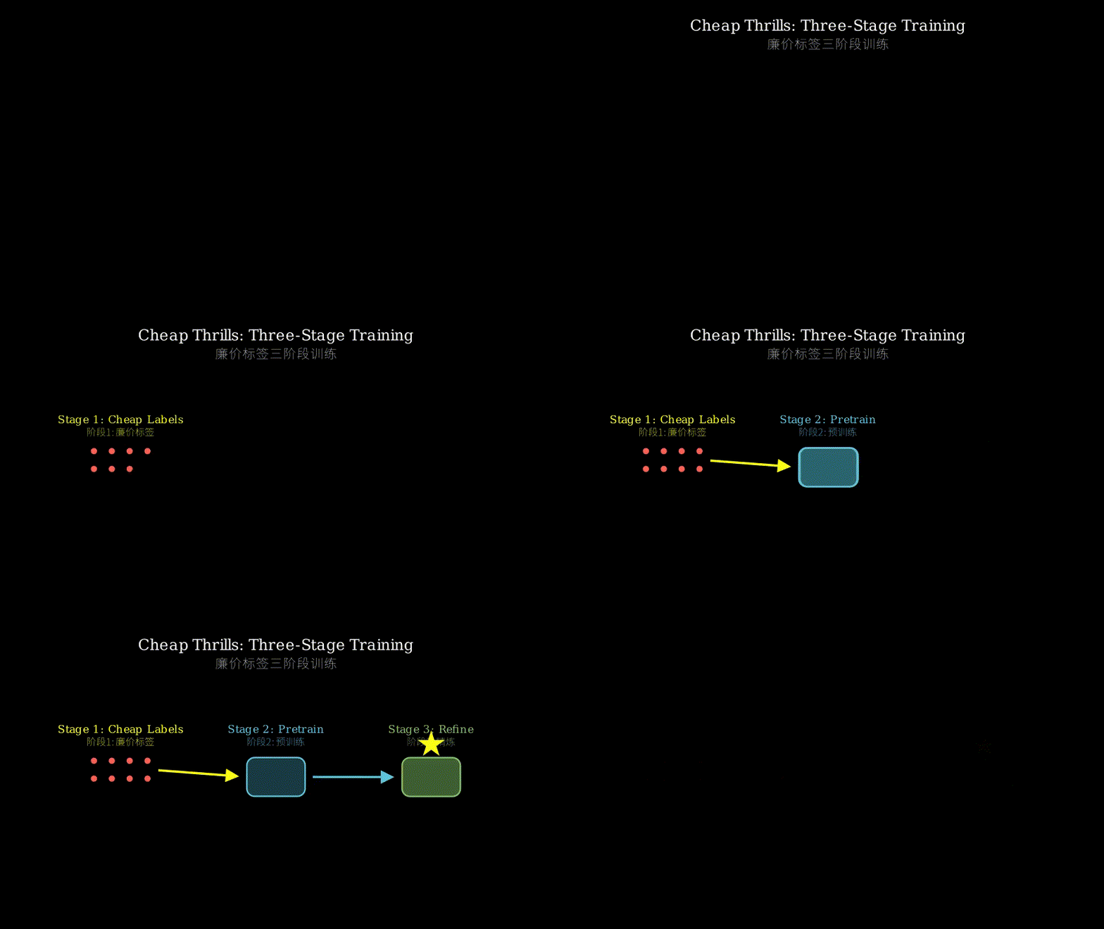
The method has three stages. Stage 1 collects cheap labels—run a fast heuristic, use a coarse solver, or even just feasible-but-suboptimal solutions. These labels are wrong, but they’re directionally correct and cost almost nothing. Stage 2 does standard supervised pretraining on these cheap labels. The model learns a rough approximation of the solution manifold. Stage 3 switches to self-supervised learning, where the model refines itself by directly optimizing the original objective and constraints.

Stage 1: Cheap Label Collection
    Problem parameters ---> [Fast heuristic] ---> Imperfect labels
                                                   (feasible but suboptimal)

Stage 2: Supervised Pretraining
    Parameters + Labels ---> [Neural net] ---> Rough approximation
                                                (near solution manifold)

Stage 3: Self-Supervised Refinement
    Parameters ---> [Pretrained net] ---> Candidate solution
                           |                      |
                           |                      v
                           |              [Evaluate objective
                           |               + constraints]
                           |                      |
                           +<-----[Backprop]------+
                                  (refine to optimality)

Think of it like learning to play darts. Stage 1 is watching someone who’s mediocre—they hit the board but rarely the bullseye. You learn the general throwing motion and where to aim. Stage 2 is practicing by copying their throws. You won’t be great, but you’ll consistently hit the board. Stage 3 is when you start keeping score yourself. You throw, see where it lands, and adjust. The key insight: you don’t need a perfect teacher to learn the basic motion. Once you’re hitting the board reliably, self-correction takes over.

The cheap labels get the model into a “basin of attraction”—a region where gradient descent can find the true optimum. The paper proves this theoretically: if your initialization is within a certain distance of the optimal solution manifold, self-supervised learning converges. The cheap labels don’t need to be good; they just need to be good enough to avoid the worst local minima.

Key Concepts

• Basin of attraction: Imagine a landscape with hills and valleys. If you’re trying to roll a ball to the lowest valley (the optimal solution), where you start matters. A basin of attraction is a region where, no matter where you drop the ball, it rolls to the same valley. Outside that region, the ball might get stuck in a different valley (local minimum). Cheap labels place your model inside the right basin—not at the bottom, but close enough that gradient descent finishes the job. Example: in power grid optimization, a cheap label might violate voltage constraints slightly, but it gets the power flow directions roughly right. That’s enough.

• Amortized optimization: Instead of solving each optimization problem from scratch, train a neural network once to instantly map problem parameters to solutions. It’s like memorizing multiplication tables instead of adding repeatedly. The upfront cost is high (training), but each query is nearly free. The challenge: the network must generalize across the entire parameter space, not just memorize specific instances.

• Self-supervised refinement: The model improves itself by directly optimizing the original problem’s objective and constraints, using its own predictions as starting points. No external labels needed—the loss function is the actual optimization objective. The danger: if you start far from the solution, gradients point in useless directions and you get stuck. That’s why pretraining with cheap labels matters.

Framework Shift

Before (mainstream approach):        After (this paper):

Option A: Supervised                 Stage 1: Cheap labels
  Expensive labels                     Fast heuristic
       |                                    |
       v                                    v
  Train model                          Stage 2: Pretrain
       |                                    |
       v                                    v
  Done (but costly)                    Stage 3: Self-supervised
                                            |
Option B: Self-supervised                  v
  Random init                          Done (cheap + accurate)
       |
       v
  Fight bad gradients
       |
       v
  Maybe converge

From “choose your poison” to “have your cake and eat it too”—the core shift is recognizing that label quality and training method are orthogonal choices, not a binary trade-off.

Expert Assessment

Problem choice: Real gap. Amortized optimization is genuinely useful for applications like power grids and robotics where you solve similar problems repeatedly. The cost-accuracy trade-off has been a practical blocker, not an academic curiosity. This sits at the intersection of optimization and ML, which is heating up.

Method maturity: Clever insight, not brute force. The three-stage structure is almost obvious in hindsight, which is the mark of good ideas. The theoretical analysis (basin of attraction criterion) provides principled guidance on when cheap labels suffice. However, the paper doesn’t deeply explore what makes a label “cheap but useful”—that’s left somewhat empirical.

Experimental integrity: Baselines are fair. They compare against pure supervised (expensive labels), pure self-supervised (no labels), and ablations of their own method. The 59x cost reduction is measured honestly—they count label generation cost, not just training time. One concern: the cheap label strategies are domain-specific (heuristics for power grids, coarse solvers for PDEs). Generalization across problem types isn’t fully explored.

Writing quality: The paper front-loads motivation well, but the theoretical section (Section 4) is dense and could use more intuition before diving into Lipschitz constants. The experimental section is thorough but repetitive—three domains with similar narratives. Condensing experiments and expanding the “when does this fail?” discussion would elevate it.

Verdict: weak accept — Solid contribution with practical impact, but the theoretical novelty is incremental and the method’s boundaries aren’t fully mapped.

Takeaways

The “basin of attraction” framing is immediately useful. If you’re training any model with self-supervised losses (physics-informed neural nets, differentiable simulators, neural optimizers), ask: “Do I need perfect initialization, or just good-enough initialization?” This paper shows that rough pretraining can substitute for careful architecture design or initialization schemes.

Specific steal: the merit-based criterion (Section 4.2) gives you a way to evaluate whether your cheap labels are sufficient without running the full training pipeline. Compute the distance between cheap labels and true solutions on a small validation set. If it’s within the basin radius, you’re good.

For practitioners in domains with expensive ground truth (molecular dynamics, climate modeling, logistics), this suggests a workflow: invest in a small set of high-quality labels for validation, generate bulk training data with fast approximations, pretrain, then refine. The paper’s power grid experiments are a template.

One caveat: the method assumes your self-supervised loss is well-behaved near the solution. If your problem has discontinuous constraints or combinatorial structure, the refinement stage might still struggle. The paper doesn’t address discrete optimization.