BiGain: Making Diffusion Models Fast Without Choosing Between Quality and Accuracy

Paper: 2603.12240 Authors: Jiacheng Liu, Shengkun Tang, Jiacheng Cui, Dongkuan Xu, Zhiqiang Shen Categories: cs.CV, cs.LG

The Gap

Diffusion models are expensive to run. Researchers have developed acceleration techniques—token merging, downsampling—that make generation faster. But here’s the catch: these methods optimize for one thing only: synthesis quality. They ignore that diffusion models are increasingly used for classification tasks too (yes, the same model can both generate images and classify them). When you speed up a diffusion model using existing methods, generation might stay good, but classification accuracy tanks.

The gap: no one has designed acceleration that respects both objectives simultaneously. Prior work treats generation and classification as separate problems requiring separate solutions.

Problem: Diffusion models slow + used for dual purposes
   |
   v
Assumption: Frequency content matters differently for generation vs classification
   |
   v
Method: Frequency-aware compression (preserve edges + semantics)
   |
   +---> Laplacian-gated token merging (generation)
   +---> KV downsampling with interpolation (classification)
   |
   v
Evidence: 7.15% accuracy gain + 0.34 FID improvement (ImageNet-1K, 70% compression)
   |
   v
Conclusion: Balanced spectral retention enables joint optimization

The Increment

One sentence: Before BiGain, accelerating diffusion models meant choosing between generation quality and classification accuracy; after BiGain, you can improve both simultaneously through frequency-aware compression.

Core Mechanism

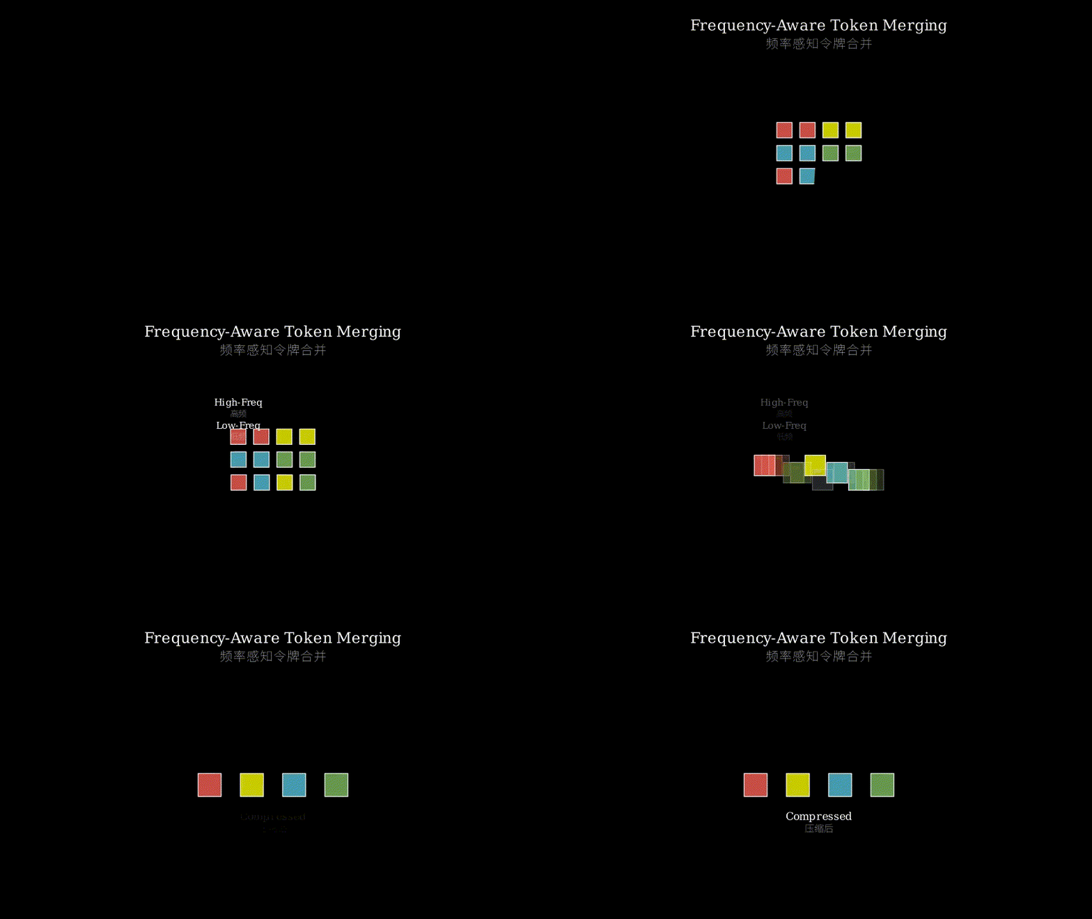
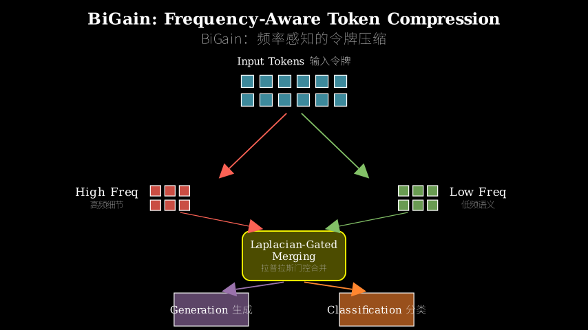
BiGain has two operators working in tandem. First, Laplacian-gated token merging analyzes each token’s frequency content using a Laplacian operator (essentially edge detection). Tokens with high-frequency content—edges, textures, fine details—get protected from merging. Tokens with low-frequency content—smooth regions, uniform areas—are candidates for merging. The gating mechanism uses this frequency score to decide merge probability.

Second, Interpolate-Extrapolate KV Downsampling targets the attention mechanism. In transformer attention, you have queries (Q), keys (K), and values (V). BiGain downsamples K and V using a controllable blend between nearest-neighbor pooling (preserves sharp features) and average pooling (captures broader context). The blend ratio is tunable. Crucially, queries stay full resolution, maintaining attention precision.

The two operators complement each other: token merging reduces the number of tokens flowing through the network (fewer computations), while KV downsampling reduces the memory footprint of attention operations (smaller matrices). Both use frequency awareness to decide what to compress and what to preserve.

Input tokens (N tokens)
   |
   v
[Laplacian operator] ---> Frequency scores
   |                           |
   v                           v
High-freq tokens         Low-freq tokens
(preserve)               (merge candidates)
   |                           |
   +----------+----------------+
              |
              v
        Merged tokens (N' tokens, N' < N)
              |
              v
        Attention layer
              |
    +---------+---------+
    |         |         |
    Q         K         V
(full res) (downsample) (downsample)
              |
              v
    [Interpolate-Extrapolate pooling]
              |
              v
        Attention output

Think of BiGain like a photo editor’s smart compression tool. When you compress a photo, you want to keep sharp edges (text, faces, boundaries) while aggressively compressing smooth areas (sky, walls). The Laplacian-gated merging is like identifying which pixels are “edge pixels” versus “smooth pixels”—you protect edges, merge smooth regions. The KV downsampling is like creating a lower-resolution reference image for color matching while keeping your selection tool (queries) at full resolution. You can still select precisely, but the reference data is compressed. The key insight: different parts of the image carry different types of information, and you compress them differently based on what downstream tasks need—generation needs edges, classification needs semantic structure.

Key Concepts

• Frequency separation in feature space: In signal processing, any signal can be decomposed into frequency components—low frequencies capture slow-changing patterns (overall shape, global structure), high frequencies capture rapid changes (edges, textures). This paper applies the same idea to neural network features. Each token in a diffusion model’s feature map has frequency content. By analyzing this content (using a Laplacian operator, which is essentially a high-pass filter), you can tell which tokens carry fine-grained detail versus coarse semantic information. Example: in an image of a cat, low-frequency tokens might represent “furry blob in center,” while high-frequency tokens represent “whisker edges” and “eye boundaries.” Generation needs those whisker edges to look realistic; classification needs the “furry blob” semantic signal.

• Laplacian operator as frequency detector: The Laplacian is a second derivative operator. In images, it responds strongly to edges and weakly to smooth regions. Mathematically, it’s the sum of second derivatives in all directions. When you apply it to a feature map, high Laplacian magnitude means “this token has high-frequency content” (edges, textures). Low magnitude means “this token is smooth” (uniform regions). BiGain uses this as a gating signal: high Laplacian score → don’t merge this token; low score → safe to merge. It’s like using a metal detector to find valuable items before compressing a storage unit—you don’t want to compress the valuable stuff.

• KV downsampling with query preservation: In transformer attention, Q·K^T produces attention weights, then weights·V produces output. If you downsample Q, K, and V equally, you lose precision everywhere. BiGain’s insight: downsample only K and V (the “database” you’re searching), keep Q at full resolution (the “search query”). This is like reducing the resolution of a map while keeping your GPS coordinates precise—you can still pinpoint locations, but the map data is compressed. The interpolate-extrapolate part means blending nearest-neighbor pooling (sharp, preserves local features) with average pooling (smooth, captures context). The blend ratio controls the trade-off between local precision and global context.

Framework Shift

Before (mainstream approach):        After (this paper):

Acceleration goal:                   Acceleration goal:
  Generation quality                   Generation + Classification
         |                                      |
         v                                      v
  Uniform compression                  Frequency-aware compression
  (merge/downsample                    (protect high-freq for generation,
   everything equally)                  preserve semantics for classification)
         |                                      |
         v                                      v
  Fast generation,                     Fast generation + accurate classification
  poor classification                  (both improved)

From uniform compression to frequency-aware compression, the core shift is recognizing that different downstream tasks need different frequency bands, so compression should be selective rather than uniform.

Expert Assessment

Problem choice: This is a real gap, not manufactured. Diffusion models are genuinely being used for both generation and classification (recent work shows they’re competitive classifiers), and acceleration is a practical necessity. The joint optimization angle is novel—prior work treated these as separate problems. It sits at the intersection of two active research threads (diffusion acceleration + diffusion-based classification), which is a smart position.

Method maturity: The frequency separation insight is clever and well-motivated. However, the execution is somewhat incremental—Laplacian operators for edge detection and KV downsampling are known techniques. The contribution is more in the combination and application context than in novel algorithmic components. I don’t see simpler approaches being overlooked; the method is reasonably direct given the problem formulation.

Experimental integrity: Baselines are fair (ToMe, DiffRate, standard downsampling). Experiments span multiple architectures (DiT, U-Net) and datasets (ImageNet-1K/100, Oxford Pets, COCO). The numbers are convincing—7.15% accuracy gain with FID improvement is substantial. One minor flag: the paper doesn’t deeply explore failure modes or cases where the method doesn’t help. But overall, the experimental work is solid.

Writing quality: The abstract is dense and jargon-heavy (“frequency-aware representation disentangles fine detail from global semantics”). The core insight—that generation needs edges and classification needs semantics—could be stated more directly upfront. The related work section is thorough but could be trimmed. If I were rewriting one section, it would be the introduction: lead with the intuition (frequency separation), then formalize.

Verdict: Weak accept—solid contribution addressing a real problem with convincing results, but the method is more clever application than fundamental innovation.

Takeaways

Practitioners can steal the frequency-aware compression principle: when optimizing for multiple objectives, analyze what information each objective needs, then compress selectively. Specifically: (1) Use Laplacian gating (or any edge detector) before token merging in vision transformers—it’s a simple addition that preserves important features. (2) In attention mechanisms, consider downsampling K/V while keeping Q full resolution—this asymmetric compression maintains precision where it matters. (3) The interpolate-extrapolate pooling idea (blending nearest and average) is a tunable knob for controlling local-vs-global trade-offs in downsampling. Beyond diffusion models, this applies anywhere you’re compressing representations for multiple downstream tasks—the key is identifying what frequency bands each task relies on.