Thinking Without Words: BDH-CQ Buys ARC Reasoning for $0.0007

Paper: 2608.09888 Authors: Björn Engdahl, Adrian Kosowski, Jan Chorowski, Zuzanna Stamirowska, Przemysław Uznański, Junlin Jiang, Rohan Phadke, Remigiusz Kinas, Richard Zhong Categories: cs.NE, cs.AI, cs.LG, stat.ML

The Gap

ARC-AGI is the benchmark where you cannot memorize your way to a good score: every task hands you two to four input/output grid pairs, and you must infer the rule and apply it to a fresh grid. Two families currently do well, and both pay for it in an awkward currency.

The first family is large language models with test-time compute. o3-class systems, long chain-of-thought sampling, and program-synthesis-over-a-DSL pipelines all reach respectable accuracy by spending tokens — sometimes tens of thousands per task, which lands anywhere from cents to tens of dollars. The reasoning is verbalized, which is nice for interpretability and terrible for cost: every intermediate thought has to be serialized through a vocabulary bottleneck and re-encoded.

The second family is the small recurrent-depth models: HRM (Hierarchical Reasoning Model, ~27M params) and TRM (Tiny Recursive Model, ~7M) get surprisingly high numbers with heavy latent recursion instead of tokens. But their setup is transductive — they train on the evaluation puzzles themselves, typically with per-puzzle embeddings and massive augmentation. There is no in-context learning happening at inference; the “learning from demonstrations” was folded into a training run. Ask them to handle a genuinely unseen task from its demos alone and the mechanism is not there.

So the gap is a missing diagonal: in-context learning (demos consumed at inference, no gradient steps) combined with latent recurrent reasoning (thinking in vectors, not tokens). BDH-CQ builds on the authors’ own BDH (“Dragon Hatchling”) architecture — sparse positive neuron activations plus local Hebbian synaptic plasticity — which happens to give you a natural place to *put what you learned from the demonstrations: the synaptic state itself.

[Problem] ARC: infer a novel rule from 2-4 demos, apply it once
    |
    +-- route A: big LLM, verbalized CoT ...... $0.05 to $10+ / task
    +-- route B: HRM / TRM latent recursion ... cheap, but TRAINED
    |                                           on the eval puzzles
    |                                           (no inference-time ICL)
    v
[Assumption] demos do not need to be re-read as tokens;
             they can be *written into recurrent state*,
             and reasoning can be *state iteration*
    |
    v
[Method] BDH-CQ = Context phase (Hebbian write of demos)
                + Query phase (T steps of latent iteration)
    |
    v
[Evidence] 150M params: 29.5% pass@2 @ ~$0.0007 / task
           + controlled ARC-like interventions
             (demo count, contradictory demos, rule consistency,
              which concepts stay hard)
    |
    v
[Conclusion] a new point below the ARC-AGI-1 cost-accuracy
             Pareto frontier; ICL without a token trace

The Increment

One sentence: Before, cheap ARC reasoners had to be trained on the puzzles they would be tested on, and genuine in-context reasoners had to talk their way to an answer; after, a 150M-parameter model absorbs demonstrations directly into its recurrent memory and thinks silently, hitting 29.5% pass@2 for less than a tenth of a cent.

Core Mechanism

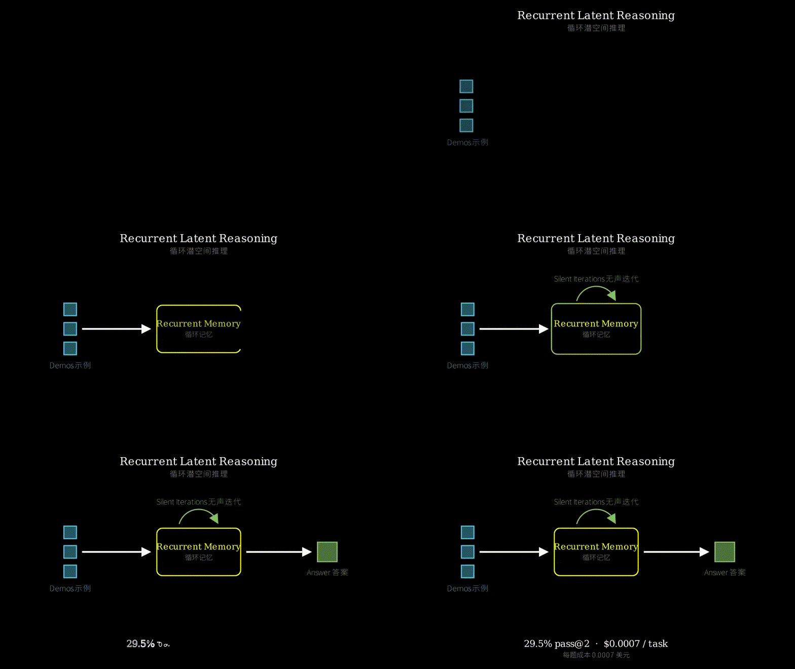
The model splits inference into two phases over the same network. In the context phase, the demonstration pairs are streamed in as a sequence. BDH’s neurons are sparse and non-negative, and co-activation drives a local Hebbian update to a synaptic state matrix — functionally a fast-weight / linear-attention-style state, but framed as plasticity between neuron pairs rather than key-value retrieval. Nothing is stored as a growing token cache; the demos are *compressed into synapses. By the end of the context phase, the state is a task-specific modulation of the network — effectively an inferred program, encoded as which pathways are now easy to traverse.

In the query phase, the query grid enters, and the network iterates. Each step, the activation vector is updated by both the slow weights (learned in pretraining, shared across all tasks) and the synaptic state written by the demos. This runs for some number of steps in latent space with no tokens emitted — there is no verbalized chain of thought to inspect. Only after the iteration settles does a decoder read out the output grid. Cost therefore scales as (FLOPs per step) × (number of steps), not as (tokens) × (context length), which is where the four-orders-of-magnitude gap comes from.

The evaluation is the other half of the contribution, and arguably the more scientifically interesting half. Because the demonstrations are a controllable input rather than baked into training, the authors can intervene: vary how many demos are shown, feed contradictory or partially-informative demos, and check whether the model applies one inferred transformation consistently across a grid or drifts region by region. That is a genuine probe of “what did it learn from the demos,” which is exactly the question transductive HRM/TRM setups cannot ask.

  demos: (in1,out1) (in2,out2) (in3,out3)      query grid
              |                                     |
              v                                     v
  +--------------------------------+   +---------------------------+
  |  CONTEXT PHASE                 |   |  QUERY PHASE              |
  |                                |   |                           |
  |  tokens ..> sparse pos. x      |   |  sigma held fixed         |
  |             (few neurons on)   |   |  loop t = 1..T:           |
  |                                |   |    x <- act( W x          |
  |  Hebbian write:                |   |            + sigma x )    |
  |    sigma <- decay*sigma        |   |    (no tokens emitted)    |
  |             + a b^T            |   |                           |
  |                                |   |  latent trajectory only   |
  +--------------------------------+   +---------------------------+
                 \                              /
                  \___ sigma = "the rule" ____ /
                                |
                                v
                        decode output grid
                                |
                                v
                    cost ~ FLOPs_step * T   (not tokens)

The metaphor: a wax tablet and a marble. The slow weights are a factory-made marble run — fixed rails, ramps, and junctions, produced once during pretraining and identical for every task. The synaptic state is a sheet of soft wax laid over the junctions. During the context phase, each demonstration is a stylus pressing grooves into that wax: co-firing neurons deepen a channel, so certain routes through the run become the path of least resistance. The wax does not record *what the demos were, only where things now flow — that is the compression.

Then the query phase drops a marble in at the top. The marble is the activation vector. It rolls through the fixed rails, but the grooves steer it, so the same run behaves differently for a symmetry task than for a counting task. Crucially, the marble is not narrated: you do not get a running commentary of “now I detect a blue square.” It goes around the loop T times, each pass refining where it sits, and only its final resting position is read out as a grid. Chain-of-thought models, by contrast, stop the marble at every junction, photograph it, describe the photo in English, and re-drop it — accurate bookkeeping, absurd overhead. And the intervention experiments are simply: press fewer grooves, press contradictory grooves, then see where the marble lands.

Key Concepts

• Fast weights (Hebbian synaptic state) as in-context memory: A transformer remembers context by keeping every past token around in a KV cache and re-attending to it — memory grows with context length, and each new token pays to look back at all of them. The alternative is to keep no list at all and instead keep a running table of *which pairs of neurons tended to fire together. If “grid contains a blue object” and “output should be rotated” co-fired while reading the demos, the synapse between those two populations strengthens. That table has fixed size no matter how long the context is, and it acts like a temporary rewiring of the network rather than a document to re-read. The trade-off is lossy: a KV cache can recover the exact 47th token; a synaptic state can only recover a blurred superposition. For ARC, where the demos matter as a rule and not as verbatim content, that trade is favorable.

• Latent recurrent reasoning (depth recurrence): Chain-of-thought gives a model more computation by making it write more words — the extra thinking rides on the token stream. Depth recurrence gives it more computation by running the same layer stack over its own hidden state N times, thinking in continuous vectors. Concretely: to decide “is this shape enclosed?”, a CoT model might write out a flood-fill in prose; a recurrent model just lets activation spread for a few more iterations. You get compute scaling without vocabulary serialization, at the price of losing the readable trace — which also means you lose the ability to catch a wrong step by reading it.

• The cost-accuracy Pareto frontier (and what pass@2 means): ARC-AGI reports accuracy against dollars per task, so a system is “on the frontier” if nothing is both cheaper and more accurate. pass@2 means the model submits two guesses and counts a win if either is right — standard for ARC, but it does roughly double the cost-per-correct-answer relative to pass@1 intuitions. 29.5% is not close to frontier-LLM accuracy (well above 70% at the top). The claim is specifically about a *new region of the frontier: at $0.0007, nothing else was anywhere near 29.5%, so the frontier curve gets pulled down and left at the cheap end.

Framework Shift

Before (mainstream approach):          After (this paper):

  demos + query as text                  demos
        |                                  |
        v                                  v
  +---------------+                 +---------------+
  |  large LLM    |                 | wax: sigma    |  <== Hebbian
  |  attends over |                 | (fixed size,  |      write
  |  full context |                 |  = the rule)  |
  +---------------+                 +---------------+
        |                                  |
        v                                  |  query
  "step 1 ...                               \   |
   step 2 ...                                v  v
   therefore ..."   <== tokens          ( loop x T in latent )
        |                                     |
        v                                     v
     answer                               answer grid

  cost ~ tokens * context             cost ~ FLOPs_step * T
  trace: readable                     trace: none
  adaptation: prompt, or per-task     adaptation: state write,
              gradient steps (TTT)                zero gradients

  ---- or the cheap-but-transductive route ----

  eval puzzles ==> TRAINING ==> per-puzzle embeddings
     (HRM / TRM: no inference-time ICL at all)

One sentence: from reasoning as text generation over a re-readable context to reasoning as state evolution over a written-once memory, the core shift is that the demonstrations stop being something you look at and become something you are temporarily rewired by.

Expert Assessment

A caveat up front: this reads as a systems-and-evaluation report in the BDH lineage, and my read of the internals is anchored on the abstract plus the earlier Dragon Hatchling work. Treat the mechanism details above as the most plausible reconstruction, not as verified from a full method section.

Problem choice: The gap is real, not manufactured. “Cheap ARC solvers exist but they train on the test puzzles” has been the field’s quiet embarrassment since HRM, and the ARC Prize team’s own re-analyses made that clear. Putting genuine inference-time ICL on the cheap end of the curve is the right target. That said, the headline framing — “state of the art in benchmark cost efficiency” — is a self-selected axis. Cost efficiency is a ratio, and ratios are easy to win by picking the cheap corner. The honest version of the claim is narrower: at three orders of magnitude below anyone else’s price point, accuracy does not collapse to near-zero the way you might expect.

Method maturity: The core insight — Hebbian fast weights are already an in-context memory, so use them as the ICL substrate instead of bolting a KV cache on — is genuinely elegant and mechanistically motivated. But it is also incremental within the authors’ own research program; BDH-CQ is BDH plus a context/query split plus an ARC training recipe. The overlooked-simpler-approach question is the one I would press hardest: how much of this is the BDH architecture specifically versus *any linear-attention or state-space recurrence (DeltaNet, Mamba, a looped linear-attention transformer) trained on the same ARC data with the same augmentation and the same latent-iteration budget? Without that ablation, “brain-inspired plasticity” and “cheap fixed-size recurrent state” are indistinguishable explanations, and the second one is much less interesting.

Experimental integrity: Two flags. First, “computed inference cost” is a modeled number, not an invoice. It presumably assumes a particular accelerator, batch size, and utilization, and it almost certainly excludes amortized training compute — which matters a lot when your method’s advantage is precisely that it front-loads work into pretraining. A $0.0007 figure derived from FLOPs × cloud-price-per-FLOP is defensible, but it is not the same species of number as an API bill, and comparing the two on one axis quietly favors the model that is not paying a provider’s margin. Second, results are on the *public ARC-AGI-1 evaluation set. That set has been available for years, hyperparameters get tuned against it, and ARC-AGI-2 with a semi-private set exists specifically to break that loop. Until there is a semi-private or ARC-AGI-2 number, 29.5% should be read as an upper-ish estimate. Also worth stating plainly: 29.5% is below published HRM/TRM numbers on the same benchmark, so the contribution rests on the ICL setting and the price, not on accuracy.

The intervention experiments are the part I would most want to read carefully, and also the part hardest to audit — they are the authors’ own synthetic constructions, so there is no shared protocol to compare against. If they are done well (contradictory demos, held-out concept categories, measured consistency of rule application across a grid), they are a template other people should copy.

Writing quality: The likely corners cut are the cost methodology and the ablations. A cost appendix that states hardware, batch size, utilization, and whether training amortization is included would convert the headline claim from marketing to science, and it costs one page. The single rewrite that would elevate the paper: an ablation table that separately isolates (a) the BDH architecture, (b) latent iteration depth T, and (c) the ICL training recipe with its augmentations. Right now a skeptical reader has to assume the recipe is doing most of the work.

Verdict: weak accept — a genuinely novel operating point with a mechanism that makes sense and an evaluation protocol worth stealing, held back by a self-chosen headline metric, a modeled rather than measured cost, and public-set-only results.

Takeaways

Things you can actually lift from this:

• Fast weights are an underused adaptation channel. If your task looks like “consume a few examples, then answer,” you have three options: put the examples in the prompt (expensive, grows with context), fine-tune per task (gradient steps at inference, LoRA juggling), or write them into a fixed-size recurrent state. The third is badly under-explored outside of ARC, and it is a good fit for personalization, few-shot classification over streaming data, and any setting where you re-answer many queries against the same small context.

• The context/query phase split is a cheap architectural pattern. Amortize the demo ingestion once, freeze the state, then run many queries against it. This is the recurrent analogue of prompt caching, but the cached object is fixed-size instead of linear in context length.

• Add compute by iterating in latent space before you add it by generating tokens. For problems that are spatial, geometric, or otherwise not naturally linguistic — grid puzzles, layout, constraint propagation, circuit-style reasoning — verbalizing intermediate steps is pure overhead. Depth recurrence buys the same extra compute without the serialization tax. Accept that you lose the readable trace, and budget for the debugging pain that follows.

• Controllable-demonstration interventions as a diagnostic. This is the most transferable methodological idea. Because the demos are an inference-time input, you can perturb them and watch behavior change: drop demos to measure sample efficiency, inject contradictions to see which one wins, hold out concept categories to map the failure surface, measure whether one rule is applied consistently across an output. Any few-shot system can be probed this way, and most are not.

• Report your cost model, not just your cost. If you are going to compete on a cost-accuracy frontier, the credibility of the whole paper rests on a number that is trivially easy to make look good. State the assumptions before someone else does it for you.