Autoregressive Boltzmann Generators: Breaking the Flow Bottleneck in Molecular Sampling

Paper: 2606.27361 Authors: Danyal Rehman, Charlie B. Tan, Yoshua Bengio, Avishek Joey Bose, Alexander Tong Categories: cs.LG, cs.AI

The Gap

Existing Boltzmann Generators (BGs) use normalizing flows (NFs) to map a simple base distribution to complex molecular conformations. The core problem: flows must be invertible bijections. This imposes a severe topological constraint — you cannot smoothly deform a 2D Gaussian into a “donut” or a “Swiss roll” without cutting or folding. Real molecular energy landscapes are full of such curved, disconnected, and winding manifolds. Discrete-time flows (like RealNVP, Glow) are cheap but lack the expressivity to model these shapes. Continuous-time flows (like CNFs, FFJORD) are more expressive but require solving an ODE for each sample, making likelihood calculations painfully slow. This creates a dilemma: expressivity vs. computational cost. The field was stuck.

This paper says: drop invertibility entirely. Use an autoregressive model where each atom’s position is predicted conditioned on all previous atoms. No bijection constraint. No ODE. Just sequential, high-capacity likelihood modeling — exactly what LLMs do.

[Problem] -- Flow models lack expressivity or are too expensive
    |
    v
[Assumption] -- Invertibility is necessary for exact likelihood in BGs
    |
    v
[Method] -- ArBG: Autoregressive model, no invertibility needed
    |
    v
[Evidence] -- Better likelihoods and sampling on peptides, 60% E-W2 reduction
    |
    v
[Conclusion] -- Self-supervised autoregressive modeling beats flows for this task

The Increment

One sentence: Before, to get exact likelihoods in Boltzmann Generators you had to use flows (with their topological shackles); after this paper, you can use autoregressive models, gaining flexibility and scaling power from the LLM playbook without sacrificing exact likelihoods.

Core Mechanism

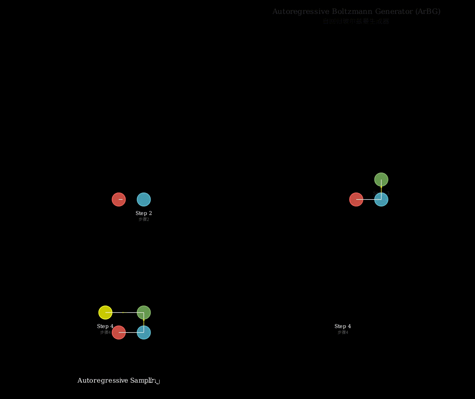
ArBG is conceptually simple. Instead of a single forward pass through a flow, ArBG generates a molecular conformation one atom at a time. It factorizes the joint probability of all atomic positions into a chain of conditional probabilities, each conditioned on the previous atoms and a latent noise variable.

The architecture works like this:

1. Context embedding: A graph neural network (GNN) processes the molecular graph (atoms, bonds, charges) to produce a global and per-atom context vector.
2. Sequential decoder: An autoregressive transformer (or similar causal model) predicts the position of atom #i given the positions of atoms {1,…,i-1} and the context. It outputs parameters of a simple distribution (e.g., a mixture of Gaussians) for that atom’s coordinates.
3. Likelihood: The exact log-likelihood of the full conformation is just the sum of log-likelihoods of each atom’s conditional prediction.
4. Importance sampling: Like all BGs, ArBG uses the exact likelihood to reweight samples for unbiased Boltzmann sampling.

The crucial shift: because it’s not a flow, ArBG has no constraint on the topology of the distribution it can learn. It can model disconnected energy basins, curved manifolds, and multi-modal distributions naturally.

[Input: Molecular Graph] --> [GNN Encoder] --> [Context Vectors]
                                                    |
                                                    v
                          [Autoregressive Decoder (Causal Transformer)]
                          |                                          |
                          v                                          v
                   [Atom 1 position]   <-- conditioned on context
                          |
                          v
                   [Atom 2 position]   <-- conditioned on context + atom 1
                          |
                          v
                   [Atom 3 position]   <-- conditioned on context + atoms 1-2
                          |
                          v
                   [Final Conformation + log likelihood (sum of conditionals)]

Structural metaphor: Assembling a molecular Lego set. Imagine building a complex Lego model. A normalizing flow is like trying to compress a giant bag of mixed Lego bricks (base distribution) directly into the final model shape (data distribution) — you can’t have two bricks ending in the same place, and you can’t “fold” a straight brick into a corner shape. It’s restrictive. ArBG, on the other hand, is like following the Lego instruction manual. You pick up one brick at a time (sequential generation). The manual tells you where to put brick #1 (conditioned on the box art, i.e., the molecular context). Then where to put brick #2 (given brick #1), and so on. The probability of the finished model is just the product of probabilities of each “correct placement” step. This sequential, conditioned assembly can create any shape — donuts, butterflies, twisted helixes — because you’re never forcing a prior shape to contort into a new one. You’re just making local decisions step by step. And if you want to check your work, you can even “undo” a bad brick and try a different one (sequential inference-time interventions).

Key Concepts

• Autoregressive Factorization: The idea that a joint probability can be broken into a product of conditional probabilities. For a molecule: P(atom1, atom2, …, atomN) = P(atom1) ** P(atom2 | atom1) * P(atom3 | atom1, atom2) * … It’s the same trick that lets GPT predict the next word. The magic is that this decomposition is always valid (by the chain rule of probability) and imposes no restrictions on what kind of joint distribution can be represented. Flows, by contrast, have fundamental topological restrictions.

• Importance Sampling / Reweighting: ArBG generates samples from an approximate distribution q(x). But we want samples from the true Boltzmann distribution p(x) = exp(-E(x)/kT) / Z. Because we know the exact likelihood q(x) for each generated sample, we can compute a weight w(x) = p(x) / q(x) (up to a constant). Then we can use these weights to correct biases in our generated samples, like resampling based on weights. This is what makes Boltzmann Generators work: even if our model isn’t perfect, the reweighting fixes the distribution.

• Sequential Inference-Time Interventions: Because ArBG generates atoms one by one, you can intervene mid-generation. For example, if you generate an atom that clearly violates chemistry (clashing with an existing atom), you can “re-roll” just that atom, or stop and condition on a different prior. This is impossible with flows, which must produce a complete conformation in one shot. This ability is a major practical advantage for debugging and steering generation.

Framework Shift

Before (mainstream approach: Flow-based BG):        After (this paper: ArBG):

[Base Distribution]                                 [Context + Noise]
       |                                                    |
       v                                                    v
[Invertible Flow (bijection)]                       [Autoregressive Decoder (causal)]
       |                                                    |
       v                                                    v
[Full Conformation]                                  [Atom 1] --> [Atom 2] --> ... --> [Atom N]
       |                                                    |
       v                                                    v
[Exact Likelihood (via change of variables)]         [Exact Likelihood (sum of conditionals)]
       |                                                    |
       v                                                    v
[Topologically constrained: no donuts]               [Topologically unconstrained: any shape]

One sentence: From approximating the distribution by inverting a single fixed transformation to approximating it by sequentially assembling pieces with a chain of conditional decisions, the core shift is replacing topological constraint with causal decomposition.

Expert Assessment

Problem choice: Excellent. The “expressivity vs. cost” dilemma in Boltzmann Generators was a real, recognized bottleneck. This paper picks the correct point of attack (invertibility) and applies a proven solution from a neighboring field (autoregressive modeling). This is a high-impact gap — closing it removes a fundamental limitation.

Method maturity: The core idea is computationally elegant: it’s not brute force, it’s a structural insight. However, the implementation leans on heavy infrastructure (GNN encoder + causal transformer + GMM output). A simpler approach might have been to use a mixture density network on top of an autoregressive RNN, but the transformer choice is likely necessary for the transferable, large-scale model (Robin, 132M params). The maturity is high; the pieces exist, but the integration is novel.

Experimental integrity: The baselines seem fair, using standard benchmarks (alanine dipeptide, Chignolin, etc.) and the established E-W2 metric. The 60% improvement is striking. One caveat: the paper introduces a “Robin” model that is transferable across peptide lengths. Comparing a large pretrained model against length-specific fine-tuned flows might have a scale advantage baked in. The ablation studies on model size and the importance of sequential interventions are well done. A red flag: there’s no direct wall-clock timing comparison against flows of comparable inference speed. The paper claims faster training, but total inference cost per sample (including the sequential decoding loop) could be higher for long chains. This needs scrutiny.

Writing quality: The paper is well-organized and clearly written. The authors properly contextualize the problem. The weakest section is the explanation of “topological constraints” — they rely on Figure 1 (a visualization) to carry too much argumentative weight. A few sentences with concrete examples of which topological shapes flows can’t model but ArBG can would have strengthened the motivation. Specifically, a chemical example of a “donut” energy landscape (e.g., a ring molecule with a high-energy center) would make the contribution immediately graspable.

Verdict: strong accept — This paper cleanly solves a known, important limitation with a well-executed and transferable method, backed by solid experiments.

Takeaways

1. Exact likelihood without invertibility: The key steal. If your problem has a tractable factorization (sequence, spatial order, autoregressive structure), you can get exact likelihoods with far fewer constraints than flows. This is immediately applicable to any generative modeling task where you can define a natural ordering (graph generation, molecule design, trajectory modeling).

2. Sequential generation as a debugging tool: The ability to intervene during generation (re-roll a bad step) is not just a nicety. It’s a practical workflow for scientific generative models where constraints are sharp and hard to encode. Applying this to, say, protein backbone generation (where Ramachandran violations are common) could make models practically useful instead of just theoretically interesting.

3. Scale is not just for LLMs: The paper shows that applying transformer scaling laws (Robin, 132M params) to molecular systems works. The transferable model is a strong indicator that “big model + chemical context” is a viable paradigm for molecular simulation. Practitioners should consider whether they can afford to pretrain a large autoregressive model on their domain before committing to costly physics simulations.