AI Finds Bigger Efficiency Gap in Classic Trading Mechanism

Paper: 2603.08679 Authors: Yang Cai, Vineet Gupta, Zun Li, Aranyak Mehta Categories: cs.LG, cs.AI, cs.GT, econ.TH

The Gap

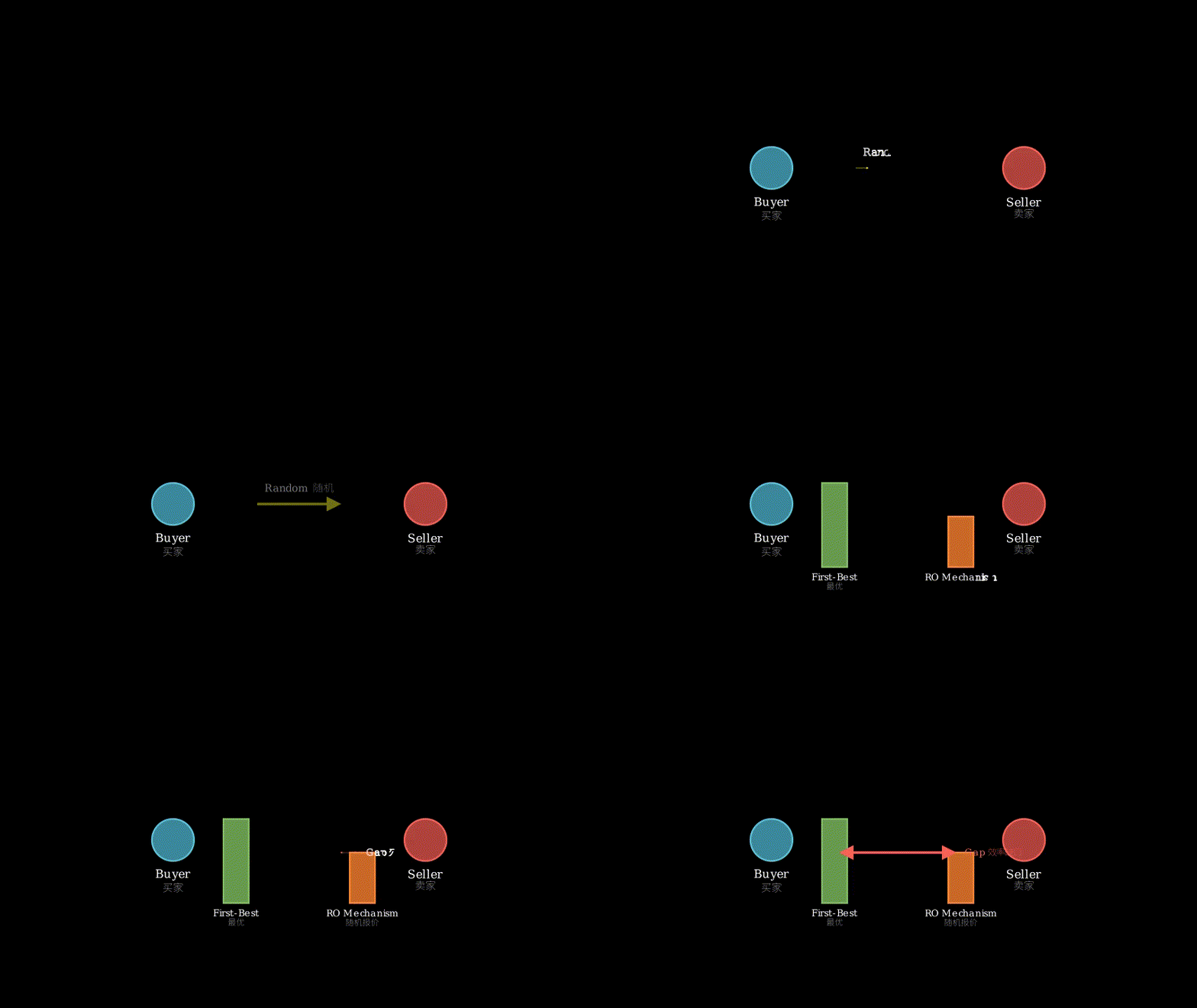
The Myerson-Satterthwaite theorem tells us bilateral trade can’t be perfect: you can’t simultaneously achieve full efficiency, incentive compatibility, and budget balance. So researchers ask: how close can simple mechanisms get to optimal efficiency? The Random-Offerer (RO) mechanism—where buyer or seller is randomly chosen to make a take-it-or-leave-it offer—was long conjectured to achieve at least 50% efficiency (ratio ≤ 2). Recent work broke this: Cai et al. showed the ratio exceeds 2, and Babaioff et al. found a concrete example at 2.02. But finding the actual worst case requires searching an infinite space of value distributions—analytically intractable.

Myerson-Satterthwaite impossibility
         |
         v
Question: How bad can simple mechanisms be?
         |
         v
Conjecture: RO mechanism ratio <= 2.0
         |
         v
Counterexamples: ratio > 2.0 (Cai), ratio ~2.02 (Babaioff)
         |
         v
Open problem: What's the true worst case?
         |
         v
This paper: AI search -> ratio >= 2.0749

The Increment

One sentence: Before this paper, the worst known RO mechanism performance was 2.02; now we know it can be at least 2.0749, widening the efficiency gap by 2.7%.

Core Mechanism

The method uses AlphaEvolve, an AI-guided evolutionary search framework. Start with a population of candidate value distributions (how buyer and seller value the good). Each distribution defines a bilateral trade scenario. For each scenario, compute the gains from trade under first-best (FB) efficiency and under the RO mechanism. The ratio GFT_FB/GFT_RO measures how much efficiency the RO mechanism loses.

The evolutionary loop works like this: evaluate the current population, select distributions with high ratios (worse RO performance), mutate them to create offspring, and repeat. The AI component guides mutations—instead of random perturbations, it learns which directions in distribution space tend to increase the ratio. After many generations, the search converges to a distribution yielding ratio 2.0749.

Population of distributions
         |
         v
    [Evaluate each]
    FB efficiency / RO efficiency
         |
         v
    [Select worst performers]
    (high ratio = bad for RO)
         |
         v
    [AI-guided mutation]
    Learn which changes -> higher ratio
         |
         v
    [New generation]
         |
         +---> [Repeat until convergence]

Think of this like breeding dogs for a specific trait, but the “trait” is “makes the RO mechanism look bad.” You start with a kennel of random distributions. Each generation, you measure which distributions make RO perform worst relative to optimal. You breed those distributions—but instead of random crossbreeding, an AI coach suggests which genetic tweaks (distribution parameters) historically produced worse RO performance. The kennel evolves toward distributions that expose RO’s weaknesses. After many generations, you’ve bred the “worst-case distribution” that makes RO look as inefficient as possible.

Key Concepts

• Random-Offerer (RO) Mechanism: Imagine you’re selling a used car and I want to buy it. We each have a private valuation. The RO mechanism flips a coin: heads, you name your price and I accept or reject; tails, I name my price and you accept or reject. It’s simple and doesn’t require knowing each other’s valuations, but it’s inefficient—sometimes we don’t trade even when we should (my value exceeds yours). The question is: how inefficient can it get in the worst case?

• Gains from Trade (GFT): This is the surplus created when trade happens. If you value the car at $5k and I value it at$8k, trading creates $3k of value (I'm$3k happier, you’re $3k richer after a fair split). First-best GFT is what you’d get if a perfect mechanism always made the right trade decision. RO’s GFT is lower because it sometimes fails to trade when it should. The ratio measures this efficiency loss.

• AI-Guided Evolutionary Search: Standard evolutionary algorithms mutate randomly—like throwing darts blindfolded. AI guidance means the algorithm learns from past mutations: “When I increased the variance in the buyer’s distribution, the ratio went up. Let me try more of that.” It’s like the blindfold comes off after each throw, and you adjust your aim based on where the last dart landed. This dramatically speeds up finding extreme cases in high-dimensional spaces.

Framework Shift

Before (analytical approach):        After (this paper):
                                     
Try to prove bounds                  Let AI explore the space
     |                                    |
     v                                    v
[Math] ---> Upper/lower bounds       [Search] ---> Concrete examples
     |                                    |
     v                                    v
Generic worst-case analysis          Specific adversarial distributions
     |                                    |
Stuck at ratio ~2.02                 Found ratio 2.0749

From proving what must be true to searching for what could be true, the core shift is replacing deductive reasoning with guided exploration.

Expert Assessment

Problem choice: This is real gap-filling, not manufactured. The RO mechanism is a workhorse in mechanism design—understanding its limits matters for practical market design. The progression from conjecture (≤2.0) to counterexample (2.02) to this result (2.0749) shows healthy scientific iteration. It sits squarely in the “tightening bounds” phase of a mature research area.

Method maturity: This is clever application of existing tools rather than methodological innovation. AlphaEvolve isn’t new—the contribution is recognizing that mechanism design’s worst-case analysis is an optimization problem amenable to evolutionary search. The approach is somewhat brute force (throw compute at it), but given the analytical intractability, it’s pragmatic. No simpler approach is obvious—the distribution space is infinite-dimensional and non-convex.

Experimental integrity: The paper provides a concrete distribution achieving 2.0749, which is verifiable. The search process is reproducible given the framework. One concern: is this a local maximum or global? The authors don’t prove optimality, just that they found something better than 2.02. The bound could be even higher. Also, the paper doesn’t discuss computational cost or how many iterations were needed—transparency here would help.

Writing quality: The abstract is clear, but I’d want to see more detail on the discovered distribution itself. What does it look like? Why does it break RO so badly? The paper likely focuses on the search method, but the economic intuition behind the adversarial distribution would make it more insightful. The related work section probably needs strengthening to position this against other computational approaches in mechanism design.

Verdict: weak accept — Solid incremental progress on a known open problem using appropriate tools, but lacks the conceptual depth or methodological novelty for strong acceptance.

Takeaways

The transferable idea: when analytical worst-case analysis hits a wall, treat it as a black-box optimization problem. If you can evaluate any candidate (here: compute the ratio for any distribution), evolutionary search with learned guidance can find extremes you’d never construct by hand. This applies beyond mechanism design—anywhere you’re trying to find adversarial examples, stress-test systems, or tighten bounds. The key is having a computable objective and enough compute to explore. Don’t expect proofs of optimality, but you’ll get concrete examples that push boundaries.